<?xml version="1.0" encoding="utf-8"?><feed xmlns="http://www.w3.org/2005/Atom" ><generator uri="https://jekyllrb.com/" version="4.4.1">Jekyll</generator><link href="/feed.xml" rel="self" type="application/atom+xml" /><link href="/" rel="alternate" type="text/html" /><updated>2026-06-01T07:57:30+00:00</updated><id>/feed.xml</id><title type="html">jdrae.github.io</title><subtitle>A personal blog built with Jekyll and hosted on GitHub Pages.</subtitle><author><name>jdrae</name><email>draejang@gmail.com</email></author><entry xml:lang="en"><title type="html">Writing Technical Blog Posts with Codex and Obsidian</title><link href="/2026/06/01/writing-tech-blog-with-codex-obsidian/" rel="alternate" type="text/html" title="Writing Technical Blog Posts with Codex and Obsidian" /><published>2026-06-01T00:00:00+00:00</published><updated>2026-06-01T00:00:00+00:00</updated><id>/2026/06/01/writing-tech-blog-with-codex-obsidian</id><content type="html" xml:base="/2026/06/01/writing-tech-blog-with-codex-obsidian/"><![CDATA[<p>I like writing. More precisely, I feel like I need to write regularly. I usually organize my thoughts in a diary, and when I learn something technical, I write it down separately in my notes.</p>

<p>So I have always thought I should create a blog and manage my writing a little more systematically. But whenever I actually set up a blog, I ended up not posting much. Eventually I would delete it, recreate it, and repeat the same cycle.</p>

<p>The reason I wrote regularly but did not upload much was simple. Once a technical post goes online, it starts to feel like a responsibility. What if I write something incorrect? What if the post looks too rough? Is this even worth publishing on a blog? Those thoughts kept following me.</p>

<p>But now, thanks to the progress of AI, I finally felt that it was time to start blogging again.</p>

<h2 id="why-a-jekyll-blog-again">Why a Jekyll blog again?</h2>

<p>Whenever I thought about a blog, I first thought of a GitHub Pages-based Jekyll blog that I could customize. The problems were that I had to build the blog myself, and managing posts was more tedious than I expected.</p>

<p>But now we are in the agent era. I described the conditions I wanted, and in a single day I was able to create something close to the blog I had imagined. Managing posts has also become much easier because an agent can help with it.</p>

<p>The conditions I wanted were fairly clear.</p>

<ul>
  <li>It should have category pages</li>
  <li>It should support toggling between Korean and English posts</li>
  <li>It should be deployable with GitHub Pages</li>
  <li>Posts should be managed as Markdown</li>
</ul>

<p>The blog is still something I am gradually improving. My next goal is to register it with Google Search Console and clean up the SEO-related settings.</p>

<h2 id="writing-starts-in-obsidian">Writing starts in Obsidian</h2>

<p>Here is the actual writing process.</p>

<p>In the past, I would have written a draft, searched for and verified details one by one, polished the sentences again, and only then published the final post. It might have taken an entire day. But now that GPT and Codex exist, I no longer need to hold every part of that process by myself.</p>

<p>I use Obsidian and Codex together to write and revise posts, and I think it works well enough that I wanted to share the process here.</p>

<p>First, I create a <code class="language-plaintext highlighter-rouge">blog</code> folder in Obsidian and add the following subfolders inside it.</p>

<div class="language-text highlighter-rouge"><div class="highlight"><pre class="highlight"><code>blog/
  raw/
  editing/
  published/
</code></pre></div></div>

<p>Each folder has a simple role.</p>

<ul>
  <li><code class="language-plaintext highlighter-rouge">raw/</code>: rough drafts that have not been polished yet.</li>
  <li><code class="language-plaintext highlighter-rouge">editing/</code>: posts currently being revised by Codex.</li>
  <li><code class="language-plaintext highlighter-rouge">published/</code>: posts that have been finalized and published to the blog.</li>
</ul>

<p>At first, I freely write the outline and the ideas I want to include in <code class="language-plaintext highlighter-rouge">raw/</code>. At this stage, writing down thoughts quickly matters more than sentence quality. It is fine if the tone is rough, and it is fine if the paragraph order is not perfect.</p>

<p>Then I add the <code class="language-plaintext highlighter-rouge">blog</code> folder as a Codex project. Codex copies the post from <code class="language-plaintext highlighter-rouge">raw/</code> into <code class="language-plaintext highlighter-rouge">editing/</code> and writes the revised version there. I ask Codex to review the style, typos, structure, Markdown formatting, and content. In other words, I use it as my own editor.</p>

<p>After reviewing the final version in <code class="language-plaintext highlighter-rouge">editing/</code>, I move it to <code class="language-plaintext highlighter-rouge">published/</code>. That keeps <code class="language-plaintext highlighter-rouge">editing/</code> as a workspace that only contains the post currently being revised.</p>

<h2 id="defining-editing-rules-with-agentsmd">Defining editing rules with AGENTS.md</h2>

<p>The most important file in this process is <code class="language-plaintext highlighter-rouge">AGENTS.md</code>.</p>

<p>If you add <code class="language-plaintext highlighter-rouge">AGENTS.md</code> to the <code class="language-plaintext highlighter-rouge">blog/</code> folder, you can define the rules Codex should follow when editing posts. For example, I wrote principles like these.</p>

<div class="language-markdown highlighter-rouge"><div class="highlight"><pre class="highlight"><code><span class="gh"># AGENTS.md</span>
<span class="p">
-</span> Codex acts as a senior editor and editor for blog posts.
<span class="p">-</span> Preserve the core content and intent of the original draft.
<span class="p">-</span> Write in polite, friendly, professional, and simple Korean.
<span class="p">-</span> Do not directly edit files inside raw/ or published/.
<span class="p">-</span> When editing a post in raw/, first copy it into editing/.
<span class="p">-</span> Make all edits only in the copied file inside editing/.
<span class="p">-</span> Normalize image links as Markdown relative links that work in Obsidian.
</code></pre></div></div>

<p>Once these rules are defined, I do not need to repeat the same instructions every time. I can simply ask, “Please edit this post.” In particular, making the roles of <code class="language-plaintext highlighter-rouge">raw/</code>, <code class="language-plaintext highlighter-rouge">editing/</code>, and <code class="language-plaintext highlighter-rouge">published/</code> explicit helps reduce the chance of accidentally modifying the original draft.</p>

<p>Everyone runs their blog differently, so the contents of <code class="language-plaintext highlighter-rouge">AGENTS.md</code> should be adjusted to fit the workflow. The important part is to clearly tell Codex what role it should play and which files it is allowed to modify.</p>

<h2 id="uploading-to-a-jekyll-blog">Uploading to a Jekyll blog</h2>

<p>Once the revision is done, it is time to upload the post to the blog.</p>

<p>I also added my personal GitHub Pages blog repository as a Codex project. Then I ask Codex to move the post into the folder where posts are stored, and to adjust the front matter and image paths to match the blog’s Jekyll format.</p>

<p>The rough flow looks like this.</p>

<ol>
  <li>Review the final post in <code class="language-plaintext highlighter-rouge">editing/</code>.</li>
  <li>Move the post into the blog repository’s <code class="language-plaintext highlighter-rouge">_posts</code> folder or the relevant post folder.</li>
  <li>Clean up the Jekyll front matter to match the blog format.</li>
  <li>Check that image paths work correctly in the deployed environment.</li>
  <li>Run a local build and check for problems.</li>
  <li>If needed, translate and create the English version as well.</li>
</ol>

<p>It is worth going through your own posting and deployment process in chat at least once. After that, you can ask Codex to “summarize the posting flow we just followed and write it into AGENTS.md,” and the process becomes much more stable the next time.</p>

<h2 id="publishing-feels-less-burdensome-now">Publishing feels less burdensome now</h2>

<p>Using this method has made publishing feel much less burdensome.</p>

<p>I can quickly write a rough draft in a stream-of-consciousness style, and typos and tone are revised according to the existing rules. Codex can suggest titles, split the post into sections, and clean up the Markdown syntax, which makes the final post much easier to read.</p>

<p>It is also useful that I can ask for verification when I am not fully confident about the content. Of course, the final responsibility still belongs to me as the person publishing the post. But it is much more efficient than struggling alone with every sentence.</p>

<h2 id="then-did-gpt-write-this-post">Then did GPT write this post?</h2>

<p>So does that mean GPT wrote this post?</p>

<p>I do not think so. When writing this post, I did not ask, “Write a blog post about how to write technical blog posts with Codex and Obsidian.” I had a topic I chose, a line of reasoning and context I had thought through, and a claim I wanted to make.</p>

<p>GPT and Codex only made the formal parts of the post easier to read. In my usage, AI is closer to an editor than an author.</p>

<p>I think this is the difference between AI slop and writing that is not. Does the writing contain the author’s thoughts and experience? If it satisfies that condition, isn’t it reasonable to get help with sentence cleanup, structure, and typo fixes?</p>

<p>I think the same idea can apply to coding. Do you know why the code was designed that way? If you can explain the reason, then even if you received help from an agent, the code is still close to something you made. An agent is not a tool that replaces my thinking. It is a tool that helps me implement the design and intent I already have more quickly and accurately.</p>]]></content><author><name>jdrae</name><email>draejang@gmail.com</email></author><category term="agentic-coding" /><category term="codex" /><category term="obsidian" /><category term="jekyll" /><category term="writing" /><summary type="html"><![CDATA[I like writing. More precisely, I feel like I need to write regularly. I usually organize my thoughts in a diary, and when I learn something technical, I write it down separately in my notes.]]></summary></entry><entry xml:lang="en"><title type="html">How Developers Without Design Knowledge Can Create Consistent UI with AI</title><link href="/2026/03/26/ai-consistent-ui-design-system/" rel="alternate" type="text/html" title="How Developers Without Design Knowledge Can Create Consistent UI with AI" /><published>2026-03-26T00:00:00+00:00</published><updated>2026-03-26T00:00:00+00:00</updated><id>/2026/03/26/ai-consistent-ui-design-system</id><content type="html" xml:base="/2026/03/26/ai-consistent-ui-design-system/"><![CDATA[<p>If someone asked me what feels most difficult when building websites or apps, the first thing that comes to mind is design.</p>

<p>In the past, I might have thought, “Isn’t functionality more important than design?” But in practice, what first catches a user’s eye is often not a “well-built feature,” but a screen that “looks well made.” That does not mean functionality is unimportant. It is simply hard to deny that what users encounter first is not code, but the interface.</p>

<p>On top of that, designers are getting increasingly good at vibe coding these days. There are so many services now that look beautiful and work well. It feels like developers are entering an era where we either need to be able to build products that look reasonably good, or create products that are clearly differentiated in functionality even if the design is lacking.</p>

<p>In any case, there is no downside to making something look good, so I started thinking it would be useful to learn at least a little about design.</p>

<h2 id="how-can-i-design-well-or-rather-make-ai-design-well">How can I design well… or rather, make AI design well?</h2>

<p>That said, studying design from the ground up in a formal way felt too inefficient for me. In this era of agents, I decided to first look for ways to “make AI design well” rather than trying to “become good at design myself.”</p>

<p>I tried Figma AI and Stitch first, but simply entering prompts did not produce satisfying results in one shot. They were fine for getting layout ideas, but it was not easy to get output polished enough to apply directly to a real service. Of course, this may have been because I was not good at writing design prompts.</p>

<p>So I watched various design methodology videos on YouTube and looked into how actual designers use AI agents.</p>

<p>That was when I came across the idea of a design system.</p>

<h2 id="the-problem-is-not-taste-but-making-things-concrete">The problem is not “taste,” but “making things concrete”</h2>

<p>After learning about design systems, I started to understand why I had been struggling. The problem was not so much that I lacked design taste, but that I could not turn the vague image in my head into concrete rules.</p>

<p>A design system is a framework that defines the design elements a service will use in advance and helps keep them consistent. For example, it defines colors, font sizes, spacing, button styles, card shapes, modal designs, and so on.</p>

<p>AI agents often produce slightly different designs each time you ask. So instead of asking them to “make it pretty” every time, I learned that if you make them refer to a predefined design system, they can produce much more consistent results.</p>

<h2 id="a-design-system-does-not-solve-ux-for-you">A design system does not solve UX for you</h2>

<p>However, I handled the screen planning myself.</p>

<p>I first drew wireframes by hand, then moved them into Figma. Since this part is related to UX, I decided it was better to think through the user flow and screen structure myself rather than hand everything over to AI.</p>

<p>A design system is closer to a tool that makes UI implementation easier. Creating a design system does not magically produce perfect UI/UX without any planning. It is much better than starting from nothing, but you still need to decide where you are headed.</p>

<h2 id="creating-and-applying-a-design-system">Creating and applying a design system</h2>

<h3 id="1-explore-references">1. Explore references</h3>

<p>
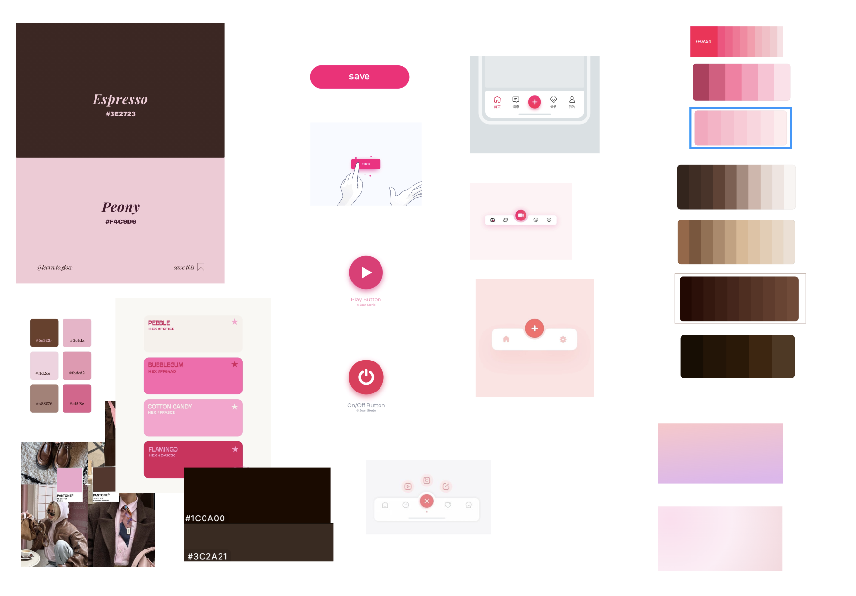
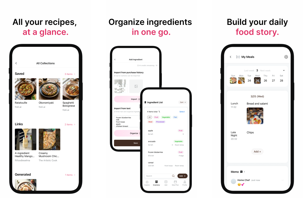
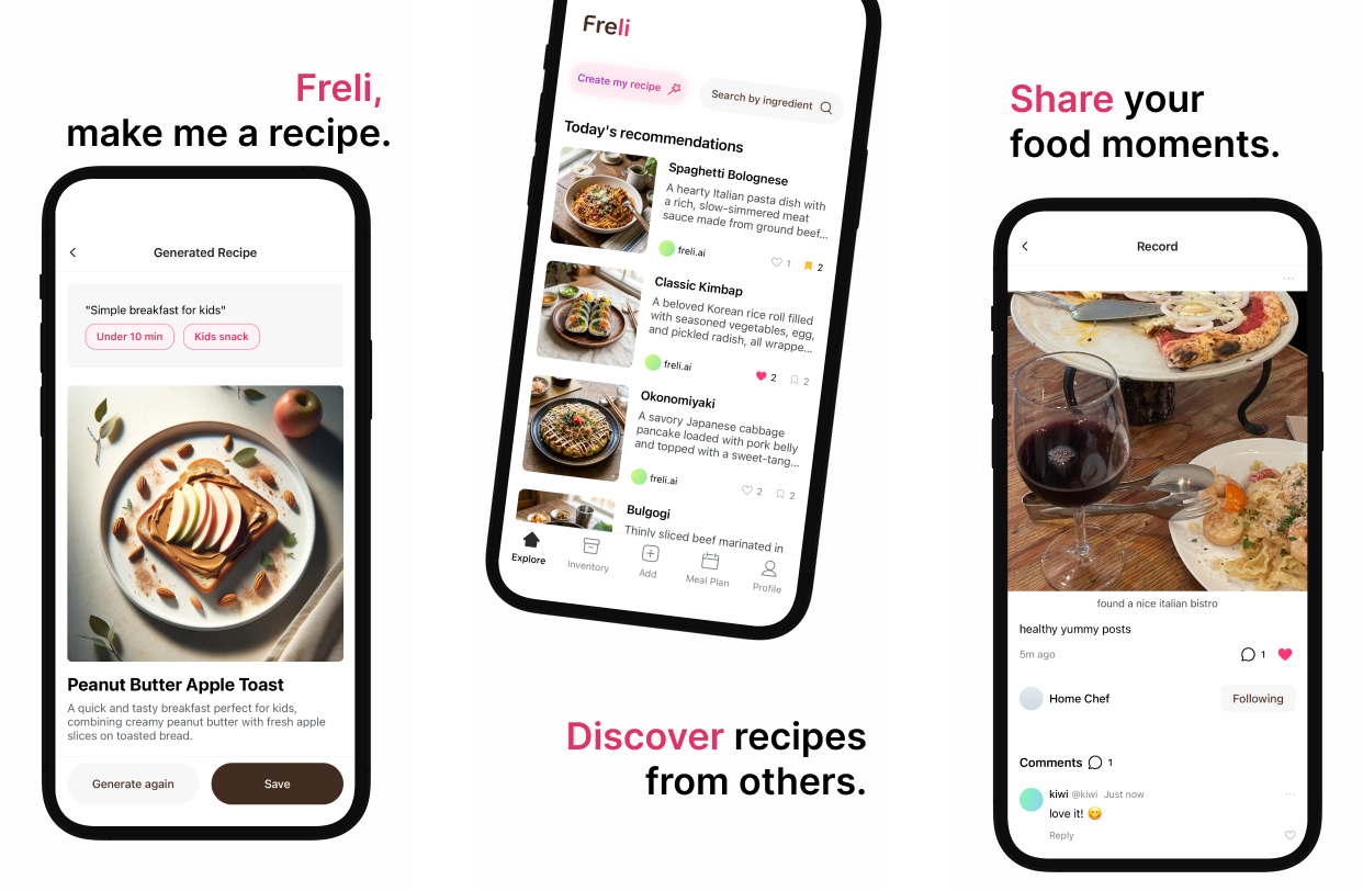
First, I decided on the mood of the app I wanted to build.</p>

<p>At minimum, it is useful to define the following:</p>

<ul>
  <li>The overall concept of the app
    <ul>
      <li>Examples: simple, analog, dark, minimal, emotional, and so on</li>
    </ul>
  </li>
  <li>Main color</li>
  <li>One or two supporting colors</li>
</ul>

<p>You can collect references from Pinterest, or look for websites and apps you want to follow. The important thing is to gather visual material that lets you confirm, “This is the kind of feeling I want.”</p>

<p>AI also needs a reference point. Just as it would be awkward to tell a person, “Please just make it pretty,” AI will also make things however it wants if you do not give it proper direction.</p>

<p><img src="/assets/images/posts/2026-03-26-ai-consistent-ui-design-system/ai-consistent-ui-reference.png" alt="Design reference example" /></p>

<h3 id="2-create-a-design-system-with-figma-mcp">2. Create a design system with Figma MCP</h3>

<p>
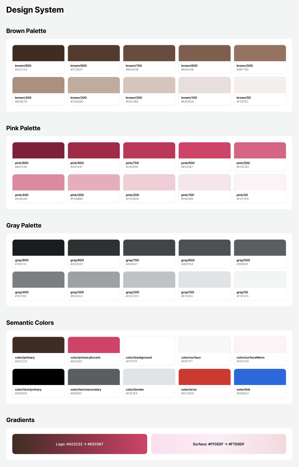
After deciding on references and the concept, I connected to Figma MCP and asked it to create a design system.</p>

<p>At this stage, I kept checking the results in Figma and making adjustments. It is also helpful to prepare basic components like buttons, modals, and cards in advance, because it makes later work much easier.</p>

<p>If you search for <code class="language-plaintext highlighter-rouge">design system prompt</code>, you can find many examples of prompts for creating design systems. I used a GitHub prompt that appeared near the top of the search results at the time.</p>

<p><a href="https://github.com/dfolloni82/design-system-prompts/blob/main/1-design-system-foundation.md#design-summary-also-provide">Design System Foundation Prompt</a></p>

<p>When creating a design system, it is good to check that it includes at least the following:</p>

<ul>
  <li>Color Token</li>
  <li>Spacing Scale</li>
  <li>Typography Scale</li>
  <li>Radius</li>
  <li>Shadow / Elevation</li>
  <li>Basic components
    <ul>
      <li>Button</li>
      <li>Input</li>
      <li>Card</li>
      <li>Modal</li>
      <li>List Item</li>
    </ul>
  </li>
  <li>States for each component
    <ul>
      <li>Default</li>
      <li>Pressed</li>
      <li>Disabled</li>
      <li>Error</li>
      <li>Loading</li>
    </ul>
  </li>
</ul>

<p><img src="/assets/images/posts/2026-03-26-ai-consistent-ui-design-system/design-system-figma-components.png" alt="Design system components organized in Figma" /></p>

<h3 id="3-turn-the-design-system-into-code-in-the-frontend-project">3. Turn the design system into code in the frontend project</h3>

<p>
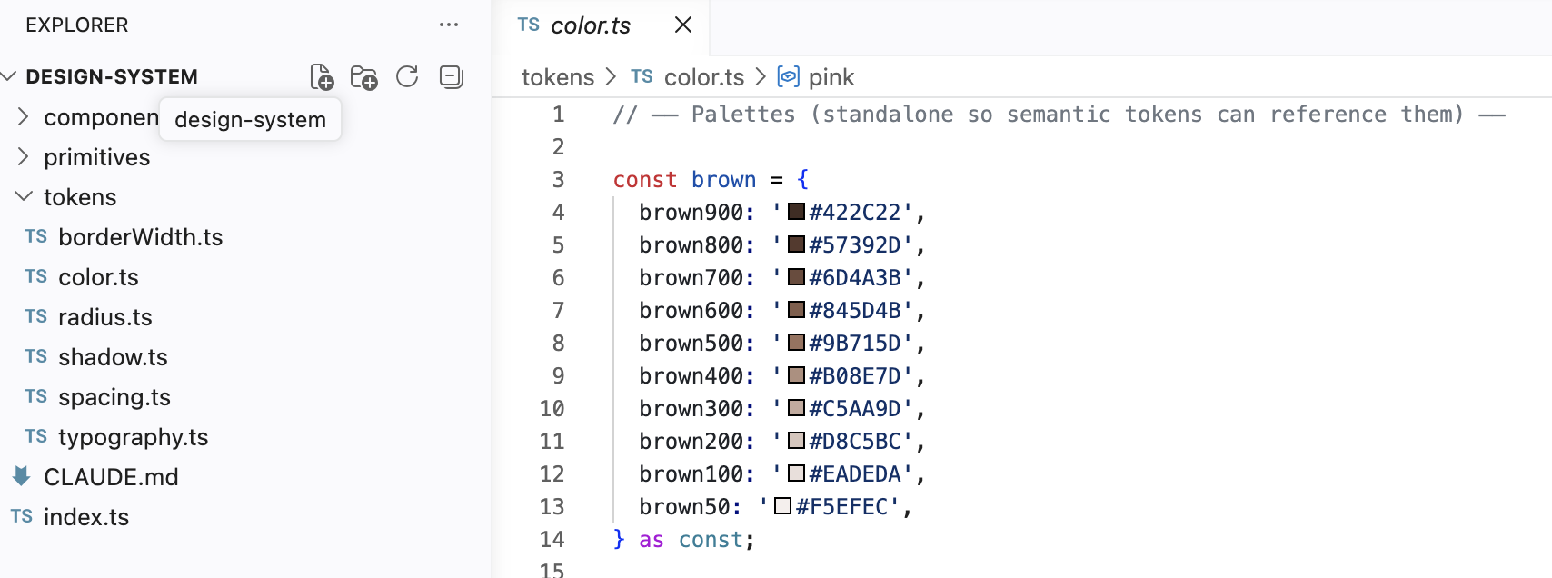
Next, I connected Figma MCP from the frontend project folder and asked it to write code based on the design system implemented in Figma.</p>

<p>The important point here is to avoid hardcoding colors, font sizes, spacing, and similar values.</p>

<p>For example, if each button directly uses a color value like <code class="language-plaintext highlighter-rouge">#3366FF</code>, you will have to search through every file later when you want to change the main color. If you manage these values as design tokens instead, you can update them in one place.</p>

<p>I also asked it to create a Markdown file defining the design system in writing. With this in place, when assigning work to an AI agent later, I can give a clear instruction such as, “Implement this based on this document.”</p>

<p><img src="/assets/images/posts/2026-03-26-ai-consistent-ui-design-system/design-system-markdown.png" alt="Design system documentation organized in Markdown" /></p>

<h3 id="4-apply-it-to-the-actual-frontend-screens">4. Apply it to the actual frontend screens</h3>

<p>Finally, I applied the code-based design system to the actual frontend screens.</p>

<p>After that, whenever I modified the screen design, I kept checking whether it matched the design system. I already had app screens that I had planned myself in Figma, and most of the structure was fixed. So I was mostly in a situation where I only needed to adjust details such as spacing, font size, and radius.</p>

<p>The advantage of this approach is that it feels less like “designing from scratch every time” and more like “refining within a defined set of rules.” It also makes instructions to AI much clearer, and the results become less inconsistent.</p>

<p><img src="/assets/images/posts/2026-03-26-ai-consistent-ui-design-system/design-system-before-application.png" alt="Screen before applying the design system" /></p>

<p><img src="/assets/images/posts/2026-03-26-ai-consistent-ui-design-system/design-system-after-application.png" alt="Screen after applying the design system" /></p>

<h2 id="additional-note-a-method-i-used-when-creating-a-landing-page">
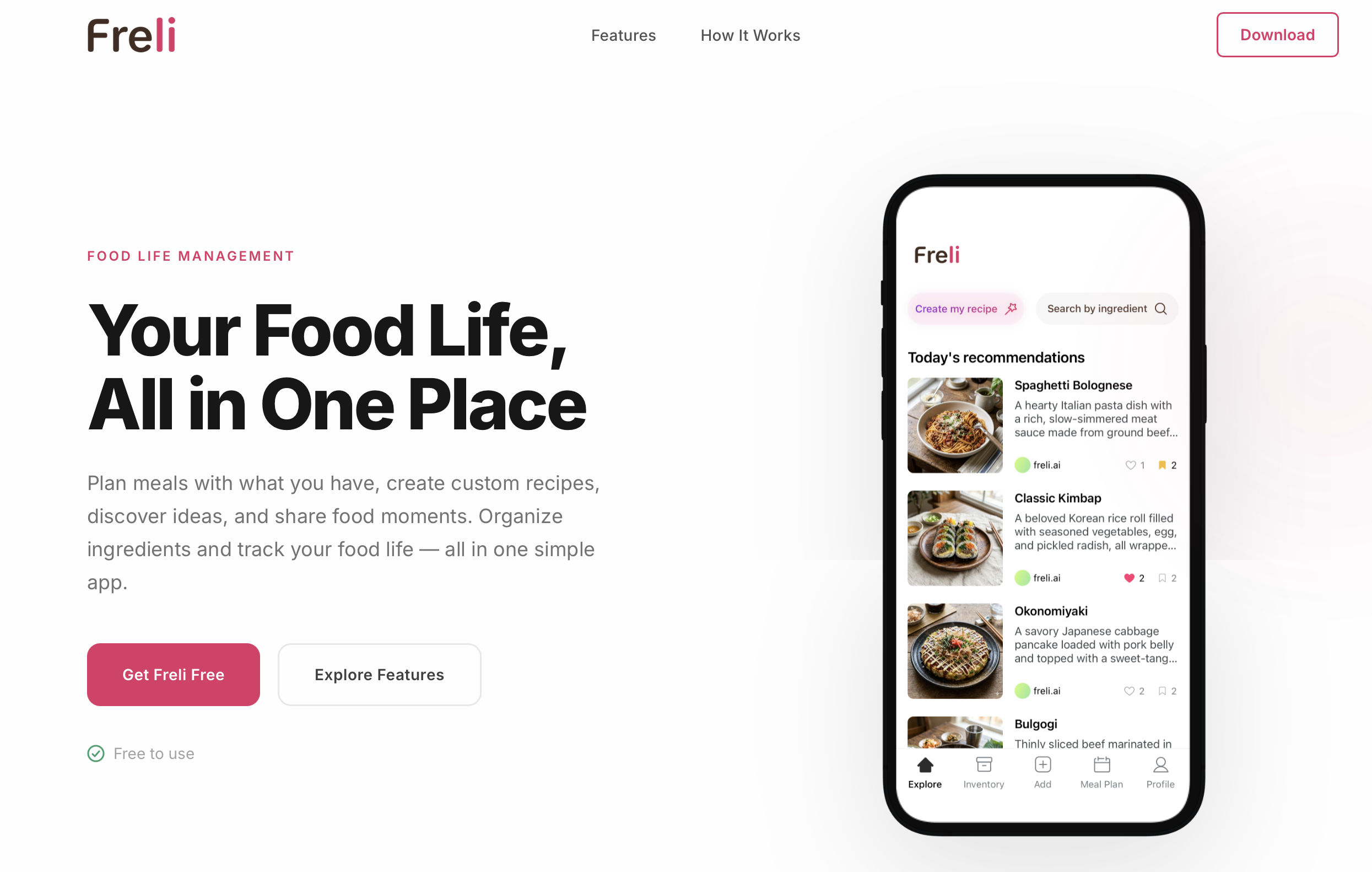
Additional note: A method I used when creating a landing page</h2>

<p>Developers often lack design knowledge, so it can be difficult to explain exactly what kind of design style they want.</p>

<p>The prompt introduced in the Reddit post below provides 25 different design styles, randomly chooses one, rewrites a detailed prompt for that style, and finally uses it to create a landing page.</p>

<p><a href="https://www.reddit.com/r/PromptEngineering/comments/1p5ztk4/i_made_a_prompt_to_generate_unique_beautiful/">Reddit - I made a prompt to generate unique beautiful landing pages</a></p>

<p>The downside of using a random approach is that you may need to try several times until you get the design you want.</p>

<p>So I first read the descriptions of the design styles defined in that prompt, chose a design philosophy I liked, and then asked AI to write a detailed prompt for that philosophy.</p>

<p>In other words, instead of immediately asking it to create a landing page, I first went through a meta-prompting process to make the design more concrete. After a few attempts, I was able to get landing pages that were closer to what I wanted.</p>

<p><img src="/assets/images/posts/2026-03-26-ai-consistent-ui-design-system/landing-page-style-prompt.png" alt="Landing page design style prompt example" /></p>

<h2 id="recommended-resources">Recommended resources</h2>

<ul>
  <li><a href="https://www.youtube.com/watch?v=nafNPuElCtY&amp;t=278s">I Built My Entire Design System in 4 Hours With AI. Full Tutorial (Claude + Cursor + Figma)</a></li>
  <li><a href="https://www.youtube.com/watch?v=sTNy6cDMEjg&amp;t=235s">How I Build a Production-Ready Design System with AI</a></li>
</ul>

<h2 id="a-video-i-found-interesting">A video I found interesting</h2>

<ul>
  <li><a href="https://www.youtube.com/watch?v=6_t66Ef0Llk&amp;t=26s">Design Systems are a Waste of Time Now</a></li>
</ul>]]></content><author><name>jdrae</name><email>draejang@gmail.com</email></author><category term="agentic-coding" /><category term="figma" /><category term="design-system" /><summary type="html"><![CDATA[If someone asked me what feels most difficult when building websites or apps, the first thing that comes to mind is design.]]></summary></entry><entry xml:lang="en"><title type="html">Notes from AWS Unicorn Day Seoul 2026</title><link href="/2026/03/19/aws-unicorn-day-seoul-2026/" rel="alternate" type="text/html" title="Notes from AWS Unicorn Day Seoul 2026" /><published>2026-03-19T00:00:00+00:00</published><updated>2026-03-19T00:00:00+00:00</updated><id>/2026/03/19/aws-unicorn-day-seoul-2026</id><content type="html" xml:base="/2026/03/19/aws-unicorn-day-seoul-2026/"><![CDATA[<p>Through several company examples and sessions, I was able to see what kinds of synergy can emerge when development with AI is combined with AWS.</p>

<p>In this post, I want to summarize the parts that stood out to me from the sessions I attended, along with key terms and concepts that came up during the talks. Since this is a reconstruction based on brief notes I took on site, some wording or details may differ slightly from the actual presentations.</p>

<hr />

<h2 id="from-implementing-text2sql-to-reducing-the-data-teams-workload-practical-operations-tips">From Implementing Text2SQL to Reducing the Data Team’s Workload: Practical Operations Tips</h2>

<blockquote>
  <p>Son Hoeyeon, Solutions Architect; Park Seoyoung, Solutions Architect (AWS)</p>

  <p>As data-driven decision-making becomes increasingly important in business settings, it is still difficult for people who do not know SQL to access data directly. This session covers how to quickly implement Text2SQL in a startup environment using LLMs, prompt engineering, and RAG, and shares practical know-how for improving accuracy in real services.</p>
</blockquote>

<h3 id="text2sql-implementation-and-operations-tips">Text2SQL implementation and operations tips</h3>

<p>When operating Text2SQL, it seemed important to design constraints and operational metrics together so that users can reliably get the results they want, rather than focusing only on the ability to convert natural language into SQL.</p>

<ol>
  <li>
    <p><strong>Constraints must be clearly defined for multi-turn queries.</strong><br />
Users often continue their questions across multiple turns, so it is important to clearly limit how much previous conversational context should be reflected and which tables and columns can be used.</p>
  </li>
  <li>
    <p><strong>Few-shot examples and schema pruning work well together.</strong><br />
Providing suitable examples to the LLM and excluding schema information that is not relevant to the query can reduce noise. As a result, you can expect more accurate and consistent SQL generation.</p>
  </li>
  <li>
    <p><strong>A/B testing should be performed based on user feedback.</strong><br />
To check whether generated SQL matches the user’s actual intent, it is necessary to collect user feedback and experimentally compare the effects of changes to prompts or model configuration.</p>
  </li>
  <li>
    <p><strong>Dynamic model selection can be considered.</strong><br />
Instead of using the same model for every query, this approach selects an appropriate model based on query difficulty, cost, and latency requirements.</p>
  </li>
</ol>

<p>For observability metrics to understand performance, you can use <strong>response time</strong>, <strong>average number of turns per session</strong>, <strong>SQL generation success rate</strong>, <strong>user feedback results</strong>, and similar indicators. In an AWS environment, Amazon Bedrock and Amazon CloudWatch can be used together to observe model calls and application operations metrics.</p>

<h3 id="terms">Terms</h3>

<ul>
  <li>
    <p><strong>Schema pruning</strong><br />
A method of selecting only the tables, columns, and relationships from the full database schema that are highly relevant to the current question and passing them to the LLM. Reducing unnecessary schema information can lower the chance that the model references the wrong table or generates incorrect joins.</p>
  </li>
  <li>
    <p><strong>Dynamic model selection</strong><br />
A strategy for dynamically choosing which model to use based on request complexity, cost, latency, and accuracy requirements. For example, simple queries can be handled by a cheaper and faster model, while complex analytical queries can be handled by a more capable model.</p>
  </li>
</ul>

<hr />

<h2 id="building-an-ontology-with-our-services-data">Building an Ontology with Our Service’s Data</h2>

<blockquote>
  <p>Park Jinwoo, Solutions Architect (AWS)</p>

  <p>This session explores ontology, a topic that many customers have recently been thinking about, and explains how to build ontology on AWS. It covers how to graph data using AWS Agentic AI services, Neptune, RDB, and analytics services, and how to add existing structured and unstructured data to an ontology. It also presents ways to use agents to remove data silos and apply the results in service, planning, and marketing.</p>
</blockquote>

<p>What is a good approach if you want to apply LLMs while effectively making use of existing database assets? In this session, one answer was <strong>ontology</strong> and <strong>graph-based data usage</strong>.</p>

<p>An ontology is a way to explicitly define the concepts, components, relationships, conditions, and entities used within a specific domain. It is also closely connected to knowledge graphs and the Semantic Web.</p>

<p>The core use cases are integrating scattered data, inferring implicit information based on relationships between data, and better understanding user intent. For example, if you manage a logistics system, you could implement a digital twin to experiment with various scenarios and use the results to suggest new processes.</p>

<p>However, there are practical barriers to data integration. It is easy to think, “Why not put all the data in one place and ask AI about it?” But in reality, “putting all the data in one place” itself is very difficult.</p>

<p>The representative reasons are as follows.</p>

<ol>
  <li>
    <p><strong>Tacit knowledge exists.</strong><br />
Knowledge such as personal experience, know-how, and intuition is difficult to turn into data because it is not clearly documented or represented in systems.</p>
  </li>
  <li>
    <p><strong>Data silos exist.</strong><br />
Different teams may use different formats, storage systems, and terminology. Even the same word, such as “user,” may have different meanings across teams.</p>
  </li>
</ol>

<p>Therefore, ontology should not be built by indiscriminately integrating all data. Instead, it is more suitable to build it by selecting the necessary data first, centered on a <strong>business objective</strong>. Final decisions should also consider the overall context rather than looking only at individual pieces of data.</p>

<p>You can organize what data to include in an ontology through questions like these:</p>

<ol>
  <li>What problem are we trying to solve?</li>
  <li>Does the data needed for that purpose actually exist?</li>
  <li>How is the data collected and loaded?</li>
  <li>How is the data currently being used?</li>
</ol>

<p>One approach introduced for implementing ontology in an AWS environment was to use the open-source SDK <strong>Strands Agents</strong> together with <strong>Amazon Neptune</strong>, AWS’s graph database. This approach can be extended into a pattern where an agent receives natural language queries, converts them into graph database queries, explores graph relationships, and then explains the results back to the user.</p>

<p>Amazon Redshift’s Zero-ETL integration also helps connect data from operational databases to analytics environments more easily, allowing fresher data to be used for analytics, AI/ML, and reporting. However, Zero-ETL does not eliminate every data transformation process, nor does it make a database immediately and perfectly understandable to an LLM. Data modeling, permissions, quality management, and business terminology still need to be designed separately.</p>

<p>It is also worth carefully deciding whether a graph DB is truly necessary when implementing an enterprise ontology. For example, travel information connects many domains such as flights, accommodation, tourism, and restaurants, so a graph DB may seem suitable. On the other hand, in actual service implementation, the join structure of an existing RDB may be easier, faster, and more intuitive.</p>

<p>In the end, I felt that the important question is not “Should we use a graph DB?” but <strong>whether the graph model provides enough value compared with the problem we are trying to solve and the complexity of the data relationships</strong>.</p>

<h3 id="terms-1">Terms</h3>

<ul>
  <li>
    <p><strong>OWL (Web Ontology Language)</strong><br />
A standard language used to express ontologies on the web. It can define classes, properties, relationships, constraints, and other elements in a machine-understandable form, and is used in Semantic Web and knowledge graph implementations.</p>
  </li>
  <li>
    <p><strong>Semantic Web</strong><br />
A concept that aims to assign meaning and relationships to information on the web so that machines, not only humans, can understand and process the meaning of data. Ontology, RDF, and OWL are often mentioned together in this context.</p>
  </li>
  <li>
    <p><strong>Digital Twin</strong><br />
A model that replicates a real-world system, device, process, or space in a digital environment. It can be used to monitor current state based on operational data or simulate what outcomes may occur under certain conditions.</p>
  </li>
  <li>
    <p><strong>Data silo</strong><br />
A state in which data is separated by department, system, or service and is not connected across boundaries. When data silos are severe, information about the same customer or product can be scattered across multiple systems, making it difficult to understand the full context.</p>
  </li>
  <li>
    <p><strong>Strands Agents</strong><br />
An open-source AI agent SDK released by AWS. It enables a model-driven approach to building AI agents and can integrate not only with AWS services such as Amazon Bedrock, but also with various external models and tools.</p>
  </li>
  <li>
    <p><strong>Zero-ETL</strong><br />
An approach intended to reduce the burden of building separate ETL pipelines and make it easier to connect data from operational data sources to analytics systems. AWS provides Zero-ETL integrations between Amazon Redshift and several data sources, with the goal of using fresher data for analytics and AI/ML.</p>
  </li>
</ul>

<h3 id="references">References</h3>

<ul>
  <li><a href="https://aws.amazon.com/ko/blogs/tech/introducing-strands-agents-an-open-source-ai-agents-sdk/">Introducing Strands Agents, an Open Source AI Agents SDK</a></li>
  <li><a href="https://builder.aws.com/content/33Y7trPz5dvINmMpzlGRS5aQZ9A/neptune-graph-analytics-using-strands-agent">Neptune Graph Analytics using Strands Agent</a></li>
</ul>

<hr />

<h2 id="building-aws-serverless-openclaw-with-vibe-coding">Building AWS Serverless OpenClaw with Vibe Coding</h2>

<blockquote>
  <p>Jung Dohyun, Principal Consultant (Roboco Co., Ltd.)</p>

  <p>This session shares practical know-how from building the Serverless-OpenClaw project in just one day by using vibe coding to migrate OpenClaw, a recent open-source project that has drawn attention, to AWS serverless infrastructure. Based on the speaker’s long experience as a software developer and technical trainer at AWS, he designed an architecture that combines Fargate, Lambda, API Gateway, and DynamoDB to maintain strong security while achieving operating costs of around $1 per month. The session covers the full process of implementing architecture design, security hardening, and cost optimization strategies through vibe coding, and introduces practical best practices such as TDD-based quality assurance, interview-based design, incremental implementation, and prompt strategies for effectively giving context to AI.</p>
</blockquote>

<p>Personally, this was the session that left the strongest impression on me. I had been used to configuring deployment steps one by one myself, so it felt especially new to learn that by using the AWS CLI, a significant portion of deployment work can be delegated to an agent.</p>

<p>Of course, entrusting deployment to an agent does not mean that every process automatically becomes safe. If anything, you need to define constraints, validation pipelines, cost ceilings, and security standards even more carefully. So in this summary, I focused more on the prompt strategy and development approach used to implement the architecture than on the architecture itself.</p>

<p>First, you need to run an interview session to design the deployment architecture according to the nature of the project. In this session, cost optimization is set as the main goal, and requirements are made concrete based on an AWS CDK stack. During the interview, various trade-offs are compared, and the maximum monthly cost suitable for the project is fixed.</p>

<p>For example, I was willing to spend up to about $20 per month on a personal project, so I was recommended a Lightsail instance. I then used Docker to run the frontend, backend, and database all on that instance. Considering future scalability, it was cheaper and easier to manage than the Railway + Vercel combination I had used before, and I was also satisfied with its performance and speed.</p>

<p>Another point that stood out to me was the validation approach. Having a person manually verify everything on every deployment is inefficient, and Human in the Loop (HIL) can become a bottleneck. Instead, it may be more realistic to have AI review things once more, receive the result as a report, and let a person perform the final check.</p>

<p>The session introduced an approach that forces every commit to pass the following validation pipeline.</p>

<ol>
  <li>
    <p><strong>TDD-based validation</strong><br />
The implementation is modified until all test cases pass.</p>
  </li>
  <li>
    <p><strong>Pre-commit hook</strong><br />
Before committing, ESLint, Vitest, type checks, and similar validations are run.</p>
  </li>
  <li>
    <p><strong>Pre-push hook</strong><br />
Before pushing to the remote repository, E2E tests and CDK Synth validation are performed.</p>
  </li>
  <li>
    <p><strong>Validation of README constraints</strong><br />
For example, it checks whether NAT Gateway usage is prohibited and whether the monthly cost ceiling is being respected.</p>
  </li>
  <li>
    <p><strong>Cost and security checklist validation</strong><br />
Skills or checklists such as <code class="language-plaintext highlighter-rouge">/cost</code> and <code class="language-plaintext highlighter-rouge">/security</code> are used to review cost and security requirements.</p>
  </li>
</ol>

<p>At first, applying this kind of validation pipeline directly may seem complicated. But if you clone the GitHub repository in the references and ask an agent, “I want to apply this validation pipeline to my project,” you can guide it to write the automation code.</p>

<h3 id="terms-2">Terms</h3>

<ul>
  <li><strong>CDK Synth</strong><br />
The process of checking whether AWS CDK code is correctly converted into a CloudFormation template. It is used to validate that infrastructure definitions are correct before deployment.</li>
</ul>

<h3 id="references-1">References</h3>

<ul>
  <li><a href="https://github.com/serithemage/serverless-openclaw">https://github.com/serithemage/serverless-openclaw</a></li>
</ul>]]></content><author><name>jdrae</name><email>draejang@gmail.com</email></author><category term="events" /><category term="aws" /><category term="text2sql" /><category term="ontology" /><category term="cdk" /><summary type="html"><![CDATA[Through several company examples and sessions, I was able to see what kinds of synergy can emerge when development with AI is combined with AWS.]]></summary></entry><entry xml:lang="en"><title type="html">Spark in Action 3: Runtime, Scheduling, and a Real-Time Processing Example</title><link href="/2025/09/08/spark-in-action-runtime-scheduling/" rel="alternate" type="text/html" title="Spark in Action 3: Runtime, Scheduling, and a Real-Time Processing Example" /><published>2025-09-08T00:00:00+00:00</published><updated>2025-09-08T00:00:00+00:00</updated><id>/2025/09/08/spark-in-action-runtime-scheduling</id><content type="html" xml:base="/2025/09/08/spark-in-action-runtime-scheduling/"><![CDATA[<p>This is the third post in my notes on Spark in Action by Petar Zečević and Marko Bonaći. In this post, I will summarize the runtime components and scheduling methods that make up a Spark application, and finally look at a real-time dashboard example.</p>

<p>While the previous posts covered RDDs, partitioning, and shuffling, this post is closer to how Spark actually runs on a cluster.</p>

<hr />

<h2 id="spark-runtime-components">Spark Runtime Components</h2>

<p>A Spark application runs through the collaboration of several runtime components.</p>

<p><img src="/assets/images/posts/2025-09-08-spark-in-action-runtime-scheduling/runtime-components-1.jpg" alt="Spark runtime component diagram 1" width="300" /></p>

<p><img src="/assets/images/posts/2025-09-08-spark-in-action-runtime-scheduling/runtime-components-2.jpg" alt="Spark runtime component diagram 2" width="300" /></p>

<h3 id="client">Client</h3>

<p>The client is the entity that starts the driver. Examples include <code class="language-plaintext highlighter-rouge">spark-submit</code>, <code class="language-plaintext highlighter-rouge">spark-shell</code>, and custom applications using the Spark API.</p>

<h3 id="driver">Driver</h3>

<p>The driver is a kind of wrapper that exists once per Spark application.</p>

<p>The driver is responsible for the following.</p>

<ul>
  <li>Request memory and CPU resources from the cluster manager.</li>
  <li>Split application logic into stages and tasks.</li>
  <li>Send tasks to multiple executors.</li>
  <li>Collect task execution results.</li>
</ul>

<p>Deployment mode can be divided into two types depending on where the driver runs.</p>

<h3 id="cluster-deployment-mode">Cluster Deployment Mode</h3>

<p>In cluster deployment mode, the driver is separated from the client.</p>

<p>The driver runs inside the cluster as a separate JVM process. Therefore, resources for the driver process, such as JVM heap memory, are managed by the cluster.</p>

<h3 id="client-deployment-mode">Client Deployment Mode</h3>

<p>In client deployment mode, the driver runs in the client’s JVM process.</p>

<h3 id="executor">Executor</h3>

<p>An executor is a JVM process that executes tasks requested by the driver and returns results back to the driver.</p>

<p>An executor runs tasks in parallel across multiple task slots. In general, task slots are implemented as threads, so they are said to be configured at around two to three times the number of CPU cores.</p>

<h3 id="sparkcontext">SparkContext</h3>

<p>SparkContext is the basic interface for accessing a Spark runtime instance. The driver creates and starts a <code class="language-plaintext highlighter-rouge">SparkContext</code> instance.</p>

<p>When running an application through the Spark API, the application must start SparkContext directly.</p>

<p>Only one SparkContext can be created per JVM. There is an option to use multiple contexts, but it is closer to a testing feature and is generally not recommended.</p>

<h2 id="scheduling">Scheduling</h2>

<p>Spark scheduling can be viewed from three perspectives.</p>

<ol>
  <li>It schedules executor, JVM process, and CPU task slot resources.</li>
  <li>The cluster manager allocates CPU and memory resources to each executor.</li>
  <li>Job scheduling is executed inside the application.</li>
</ol>

<h2 id="cluster-resource-scheduling">Cluster Resource Scheduling</h2>

<p>Cluster resource scheduling is the process of allocating resources to executors of multiple Spark applications running on a single cluster.</p>

<p>The cluster manager starts, stops, and restarts processes, and limits the maximum number of CPU cores available to each executor.</p>

<p>The cluster manager does the following.</p>

<ul>
  <li>Starts executor processes requested by the driver.</li>
  <li>Starts the driver process as well when using cluster deployment mode.</li>
</ul>

<p>Executors are not shared between applications. Therefore, if multiple applications run simultaneously on a single cluster, resource contention can occur.</p>

<h2 id="spark-job-scheduling">Spark Job Scheduling</h2>

<p>Spark job scheduling is the process of scheduling CPU and memory resources for running tasks inside a single Spark application.</p>

<p>The driver has several scheduler objects. Once executors are running, it decides which executor will run which task.</p>

<p>Multiple jobs sharing the same SparkContext compete for executor resources. SparkContext is thread-safe.</p>

<p>Job scheduling determines CPU resource usage in the cluster. It also indirectly affects memory usage, because running more tasks in a single JVM uses more heap memory.</p>

<p>CPU resources are managed at the task level. Memory resources, on the other hand, are managed by dividing them into multiple segments.</p>

<h3 id="fifo-scheduler">FIFO Scheduler</h3>

<p>The FIFO scheduler lets the job that requested resources first occupy as many task slots as it needs.</p>

<p>If the job that started first does not use many resources, other jobs can also run simultaneously. But if the first job needs to occupy all resources, the next job must wait until the existing job has used them.</p>

<h3 id="fair-scheduler">FAIR Scheduler</h3>

<p>The FAIR scheduler distributes resources evenly in a round-robin manner.</p>

<p>Even if a job requests task slots later, it does not necessarily have to wait until a long-running job completes.</p>

<p>Using scheduler pools allows weights and minimum shares to be configured. If a weight is set, jobs in a particular pool can receive more resources than jobs in other pools. The minimum share is the minimum number of CPU cores that each pool can always use.</p>

<h3 id="speculative-execution">Speculative Execution</h3>

<p>Speculative execution is a feature for reducing the problem of straggler tasks, which take unusually longer than other tasks in the same stage.</p>

<p>Spark can request the same task processing the same partition data on another executor as well. If the existing task is delayed and the speculative task completes first, Spark uses the result of the speculative task to reduce overall job latency.</p>

<p>Related settings include the following.</p>

<ul>
  <li><code class="language-plaintext highlighter-rouge">spark.speculation = true</code>: enables speculative execution.</li>
  <li><code class="language-plaintext highlighter-rouge">spark.speculation.interval</code>: the interval for checking whether speculative tasks should be launched.</li>
  <li><code class="language-plaintext highlighter-rouge">spark.speculation.quantile</code>: the progress ratio of tasks that must be completed before speculative tasks are launched.</li>
  <li><code class="language-plaintext highlighter-rouge">spark.speculation.multiplier</code>: the criterion for determining how delayed an existing task is.</li>
</ul>

<p>However, speculative tasks must be used carefully. For example, if the task writes data to a database, the same data may be written twice.</p>

<h2 id="data-locality">Data Locality</h2>

<p>Data locality is a strategy for running tasks on executors located as close as possible to the data.</p>

<h3 id="preferred-locations">Preferred Locations</h3>

<p>Spark has hostnames or executor lists that store partition data for each partition. It can use this location information to run computation close to the data.</p>

<p>However, preferred location information is available only for RDDs created from HDFS data and cached RDDs.</p>

<p>HDFS RDDs retrieve location information from the HDFS cluster through the Hadoop API. For cached RDDs, Spark directly manages the executor locations where each partition is cached.</p>

<h3 id="data-locality-levels">Data Locality Levels</h3>

<p>When Spark cannot secure the best task slot, it waits for a certain amount of time. If it still cannot secure one, it tries scheduling to the next-best location.</p>

<p>Depending on where a task runs, data locality levels are divided as follows.</p>

<ul>
  <li><code class="language-plaintext highlighter-rouge">PROCESS_LOCAL</code>: runs on the executor that cached the partition.</li>
  <li><code class="language-plaintext highlighter-rouge">NODE_LOCAL</code>: runs on a node that can directly access the partition. This is a location that can access the data without going through the network, and another executor on the same machine may fall into this category.</li>
  <li><code class="language-plaintext highlighter-rouge">RACK_LOCAL</code>: runs on another machine mounted in the same rack as the machine storing the partition. Since only YARN can refer to rack information in the cluster, this level is possible only on YARN.</li>
  <li><code class="language-plaintext highlighter-rouge">NO_PREF</code>: no preferred location exists. The data can be accessed at the same speed from anywhere in the cluster.</li>
  <li><code class="language-plaintext highlighter-rouge">ANY</code>: runs the task in another location when data locality cannot be secured.</li>
</ul>

<p>Here, a rack is a standard-sized frame for mounting servers and network equipment. Within the same rack, even if data is transferred over the network, it only needs to pass through the switch.</p>

<h2 id="memory-scheduling">Memory Scheduling</h2>

<p>Memory scheduling is the process in which the cluster manager allocates memory to executor JVM processes, and Spark manages memory used by jobs and tasks.</p>

<h3 id="memory-managed-by-the-cluster-manager">Memory Managed by the Cluster Manager</h3>

<p>The memory allocated to an executor is configured with <code class="language-plaintext highlighter-rouge">spark.executor.memory</code>.</p>

<h3 id="memory-managed-by-spark">Memory Managed by Spark</h3>

<p>In Spark 1.5.2 and earlier, executor memory was divided to store cached data and temporary shuffle data. Because usage in the divided memory regions could exceed their limits, a safety ratio was defined. The default allocation used 54% for cache, 16% for shuffling, and the remaining 30% for other Java objects and resource storage.</p>

<p>Starting with Spark 1.6.0, memory is managed in a unified way. Therefore, if there is no shuffling, the cache may occupy the entire memory. However, the area occupied by execution memory cannot be converted into the storage memory area.</p>

<h2 id="example-real-time-dashboard">Example: Real-Time Dashboard</h2>

<p>Finally, I will summarize a real-time dashboard example.</p>

<p><img src="/assets/images/posts/2025-09-08-spark-in-action-runtime-scheduling/realtime-dashboard.jpg" alt="Real-time dashboard example" width="600" /></p>

<div class="language-python highlighter-rouge"><div class="highlight"><pre class="highlight"><code><span class="k">class</span> <span class="nc">KafkaProducerWrapper</span><span class="p">(</span><span class="nb">object</span><span class="p">):</span>
    <span class="n">producer</span> <span class="o">=</span> <span class="bp">None</span>

    <span class="nd">@staticmethod</span>
    <span class="k">def</span> <span class="nf">getProducer</span><span class="p">(</span><span class="n">brokerList</span><span class="p">):</span>
        <span class="k">if</span> <span class="n">KafkaProducerWrapper</span><span class="p">.</span><span class="n">producer</span> <span class="o">==</span> <span class="bp">None</span><span class="p">:</span>
            <span class="n">KafkaProducerWrapper</span><span class="p">.</span><span class="n">producer</span> <span class="o">=</span> <span class="nc">KafkaProducer</span><span class="p">(</span>
                <span class="n">bootstrap_servers</span><span class="o">=</span><span class="n">brokerList</span><span class="p">,</span>
                <span class="n">key_serializer</span><span class="o">=</span><span class="nb">str</span><span class="p">.</span><span class="n">encode</span><span class="p">,</span>
                <span class="n">value_serializer</span><span class="o">=</span><span class="nb">str</span><span class="p">.</span><span class="n">encode</span>
            <span class="p">)</span>
        <span class="k">return</span> <span class="n">KafkaProducerWrapper</span><span class="p">.</span><span class="n">producer</span>

<span class="k">if</span> <span class="n">__name__</span> <span class="o">==</span> <span class="sh">"</span><span class="s">__main__</span><span class="sh">"</span><span class="p">:</span>
    <span class="c1"># ... omitted
</span>
    <span class="c1"># data key types for the output map
</span>    <span class="n">SESSION_COUNT</span> <span class="o">=</span> <span class="sh">"</span><span class="s">SESS</span><span class="sh">"</span>
    <span class="n">REQ_PER_SEC</span> <span class="o">=</span> <span class="sh">"</span><span class="s">REQ</span><span class="sh">"</span>
    <span class="n">ERR_PER_SEC</span> <span class="o">=</span> <span class="sh">"</span><span class="s">ERR</span><span class="sh">"</span>
    <span class="n">ADS_PER_SEC</span> <span class="o">=</span> <span class="sh">"</span><span class="s">AD</span><span class="sh">"</span>

    <span class="n">requests</span> <span class="o">=</span> <span class="n">reqsPerSecond</span><span class="p">.</span><span class="nf">map</span><span class="p">(</span><span class="k">lambda</span> <span class="n">sc</span><span class="p">:</span> <span class="p">(</span><span class="n">sc</span><span class="p">[</span><span class="mi">0</span><span class="p">],</span> <span class="p">{</span><span class="n">REQ_PER_SEC</span><span class="p">:</span> <span class="n">sc</span><span class="p">[</span><span class="mi">1</span><span class="p">]}))</span>
    <span class="n">errors</span> <span class="o">=</span> <span class="n">errorsPerSecond</span><span class="p">.</span><span class="nf">map</span><span class="p">(</span><span class="k">lambda</span> <span class="n">sc</span><span class="p">:</span> <span class="p">(</span><span class="n">sc</span><span class="p">[</span><span class="mi">0</span><span class="p">],</span> <span class="p">{</span><span class="n">ERR_PER_SEC</span><span class="p">:</span> <span class="n">sc</span><span class="p">[</span><span class="mi">1</span><span class="p">]}))</span>
    <span class="n">finalSessionCount</span> <span class="o">=</span> <span class="n">sessionCount</span><span class="p">.</span><span class="nf">map</span><span class="p">(</span>
        <span class="k">lambda</span> <span class="n">c</span><span class="p">:</span> <span class="p">(</span>
            <span class="nf">long</span><span class="p">((</span><span class="n">datetime</span><span class="p">.</span><span class="nf">now</span><span class="p">()</span> <span class="o">-</span> <span class="n">zerotime</span><span class="p">).</span><span class="nf">total_seconds</span><span class="p">()</span> <span class="o">*</span> <span class="mi">1000</span><span class="p">),</span>
            <span class="p">{</span><span class="n">SESSION_COUNT</span><span class="p">:</span> <span class="n">c</span><span class="p">}</span>
        <span class="p">)</span>
    <span class="p">)</span>
    <span class="n">ads</span> <span class="o">=</span> <span class="n">adsPerSecondAndType</span><span class="p">.</span><span class="nf">map</span><span class="p">(</span>
        <span class="k">lambda</span> <span class="n">stc</span><span class="p">:</span> <span class="p">(</span><span class="n">stc</span><span class="p">[</span><span class="mi">0</span><span class="p">][</span><span class="mi">0</span><span class="p">],</span> <span class="p">{</span><span class="n">ADS_PER_SEC</span> <span class="o">+</span> <span class="sh">"</span><span class="s">#</span><span class="sh">"</span> <span class="o">+</span> <span class="n">stc</span><span class="p">[</span><span class="mi">0</span><span class="p">][</span><span class="mi">1</span><span class="p">]:</span> <span class="n">stc</span><span class="p">[</span><span class="mi">1</span><span class="p">]})</span>
    <span class="p">)</span>

    <span class="c1"># all the streams are unioned and combined
</span>    <span class="n">finalStats</span> <span class="o">=</span> <span class="n">finalSessionCount</span> \
        <span class="p">.</span><span class="nf">union</span><span class="p">(</span><span class="n">requests</span><span class="p">)</span> \
        <span class="p">.</span><span class="nf">union</span><span class="p">(</span><span class="n">errors</span><span class="p">)</span> \
        <span class="p">.</span><span class="nf">union</span><span class="p">(</span><span class="n">ads</span><span class="p">)</span> \
        <span class="p">.</span><span class="nf">reduceByKey</span><span class="p">(</span><span class="k">lambda</span> <span class="n">m1</span><span class="p">,</span> <span class="n">m2</span><span class="p">:</span> <span class="nf">dict</span><span class="p">(</span><span class="n">m1</span><span class="p">.</span><span class="nf">items</span><span class="p">()</span> <span class="o">+</span> <span class="n">m2</span><span class="p">.</span><span class="nf">items</span><span class="p">()))</span>

    <span class="k">def</span> <span class="nf">sendMetrics</span><span class="p">(</span><span class="n">itr</span><span class="p">):</span>
        <span class="k">global</span> <span class="n">brokerList</span>
        <span class="n">prod</span> <span class="o">=</span> <span class="n">KafkaProducerWrapper</span><span class="p">.</span><span class="nf">getProducer</span><span class="p">([</span><span class="n">brokerList</span><span class="p">])</span>
        <span class="k">for</span> <span class="n">m</span> <span class="ow">in</span> <span class="n">itr</span><span class="p">:</span>
            <span class="n">mstr</span> <span class="o">=</span> <span class="sh">"</span><span class="s">,</span><span class="sh">"</span><span class="p">.</span><span class="nf">join</span><span class="p">([</span><span class="nf">str</span><span class="p">(</span><span class="n">x</span><span class="p">)</span> <span class="o">+</span> <span class="sh">"</span><span class="s">-&gt;</span><span class="sh">"</span> <span class="o">+</span> <span class="nf">str</span><span class="p">(</span><span class="n">m</span><span class="p">[</span><span class="mi">1</span><span class="p">][</span><span class="n">x</span><span class="p">])</span> <span class="k">for</span> <span class="n">x</span> <span class="ow">in</span> <span class="n">m</span><span class="p">[</span><span class="mi">1</span><span class="p">]])</span>
            <span class="n">prod</span><span class="p">.</span><span class="nf">send</span><span class="p">(</span>
                <span class="n">statsTopic</span><span class="p">,</span>
                <span class="n">key</span><span class="o">=</span><span class="nf">str</span><span class="p">(</span><span class="n">m</span><span class="p">[</span><span class="mi">0</span><span class="p">]),</span>
                <span class="n">value</span><span class="o">=</span><span class="nf">str</span><span class="p">(</span><span class="n">m</span><span class="p">[</span><span class="mi">0</span><span class="p">])</span> <span class="o">+</span> <span class="sh">"</span><span class="s">:(</span><span class="sh">"</span> <span class="o">+</span> <span class="n">mstr</span> <span class="o">+</span> <span class="sh">"</span><span class="s">)</span><span class="sh">"</span>
            <span class="p">)</span>
        <span class="n">prod</span><span class="p">.</span><span class="nf">flush</span><span class="p">()</span>

    <span class="c1"># Each partition uses its own Kafka producer to send formatted messages.
</span>    <span class="n">finalStats</span><span class="p">.</span><span class="nf">foreachRDD</span><span class="p">(</span><span class="k">lambda</span> <span class="n">rdd</span><span class="p">:</span> <span class="n">rdd</span><span class="p">.</span><span class="nf">foreachPartition</span><span class="p">(</span><span class="n">sendMetrics</span><span class="p">))</span>

    <span class="nf">print</span><span class="p">(</span><span class="sh">"</span><span class="s">Starting the streaming context... Kill me with ^C</span><span class="sh">"</span><span class="p">)</span>

    <span class="n">ssc</span><span class="p">.</span><span class="nf">start</span><span class="p">()</span>
    <span class="n">ssc</span><span class="p">.</span><span class="nf">awaitTermination</span><span class="p">()</span>
</code></pre></div></div>

<p>In this example, the number of active sessions is processed in one-second mini-batches, so results keyed by per-second timestamps are combined and sent to Kafka.</p>

<p>The Kafka producer object initialized in the driver cannot be sent to workers. Instead, the producer is initialized inside tasks that run on workers.</p>

<p>Scala’s <code class="language-plaintext highlighter-rouge">KafkaProducerWrapper</code> companion object creates a single instance through lazy instantiation and initializes a single Kafka producer instance.</p>

<p>Using <code class="language-plaintext highlighter-rouge">foreachPartition</code>, a producer object can be initialized once per JVM and used to send messages to Kafka. Since multiple partitions share the same executor JVM, the producer object can also be shared.</p>

<h2 id="closing">Closing</h2>

<p>In this post, I summarized Spark runtime components, resource scheduling, data locality, memory scheduling, and a real-time dashboard example.</p>]]></content><author><name>jdrae</name><email>draejang@gmail.com</email></author><category term="data-engineering" /><category term="spark" /><category term="scheduling" /><category term="data-locality" /><category term="streaming" /><summary type="html"><![CDATA[This is the third post in my notes on Spark in Action by Petar Zečević and Marko Bonaći. In this post, I will summarize the runtime components and scheduling methods that make up a Spark application, and finally look at a real-time dashboard example.]]></summary></entry><entry xml:lang="en"><title type="html">Spark in Action 2: Understanding Partitioning and Shuffling</title><link href="/2025/08/29/spark-in-action-partitioning-shuffle/" rel="alternate" type="text/html" title="Spark in Action 2: Understanding Partitioning and Shuffling" /><published>2025-08-29T00:00:00+00:00</published><updated>2025-08-29T00:00:00+00:00</updated><id>/2025/08/29/spark-in-action-partitioning-shuffle</id><content type="html" xml:base="/2025/08/29/spark-in-action-partitioning-shuffle/"><![CDATA[<p>This is the second post in my notes on Spark in Action by Petar Zečević and Marko Bonaći. In the first post, I looked at Spark’s basic execution flow and RDDs. In this post, I will summarize partitioning and shuffling, which directly affect performance.</p>

<p>Understanding how partitions are divided in Spark and when data movement occurs makes it much easier to see why a job becomes slow.</p>

<hr />

<h2 id="data-partitioning">Data Partitioning</h2>

<p>Partitioning is the process of splitting data across multiple cluster nodes. In Spark, partitioning has a major impact on performance and resource usage.</p>

<p>An RDD partition is a subset of RDD data. Spark splits files into partitions and stores them across cluster nodes, and the set of these distributed partitions forms a single RDD.</p>

<p>The number of partitions affects how work is distributed across the cluster. It is also directly connected to the number of tasks created when transformation operations are executed on an RDD.</p>

<p>If there are too few partitions, the cluster cannot be fully utilized. Conversely, each task may have to process too much data and exceed the executor’s memory resources.</p>

<p>In general, it is said to be good to use three to four times as many partitions as the number of cores in the cluster. However, if there are too many tasks, task management itself can become a bottleneck.</p>

<h2 id="partitioner">Partitioner</h2>

<p>A <code class="language-plaintext highlighter-rouge">Partitioner</code> performs partitioning by assigning a partition number to each element of an RDD.</p>

<h3 id="hashpartitioner">HashPartitioner</h3>

<p><code class="language-plaintext highlighter-rouge">HashPartitioner</code> is the default partitioner. It calculates the partition using each element’s Java hash code with the formula <code class="language-plaintext highlighter-rouge">partitionIndex = hashCode % numOfPartitions</code>.</p>

<p>Because it is hash-based, it cannot guarantee that all partitions will be exactly the same size. However, as long as the number of partitions is not too small, the data is generally distributed fairly evenly.</p>

<h3 id="rangepartitioner">RangePartitioner</h3>

<p><code class="language-plaintext highlighter-rouge">RangePartitioner</code> splits data in a sorted RDD into roughly equal range intervals. It determines range boundaries based on sampled data.</p>

<p>The book explains that it is not often used in practice.</p>

<h3 id="custom-partitioner-for-pair-rdds">Custom Partitioner for Pair RDDs</h3>

<p>When processing Pair RDDs composed of key-value pairs, a custom <code class="language-plaintext highlighter-rouge">Partitioner</code> can be used. It is useful when data must be placed into specific partitions according to a particular criterion.</p>

<h2 id="shuffling">Shuffling</h2>

<p>Shuffling refers to physical data movement between partitions.</p>

<p>Shuffling occurs when data from multiple partitions must be combined to create partitions for a new RDD.</p>

<div class="language-scala highlighter-rouge"><div class="highlight"><pre class="highlight"><code><span class="k">val</span> <span class="nv">prods</span> <span class="k">=</span> <span class="nv">transByCust</span><span class="o">.</span><span class="py">aggregateByKey</span><span class="o">(</span><span class="nc">List</span><span class="o">[</span><span class="kt">String</span><span class="o">]())(</span>
  <span class="o">(</span><span class="n">prods</span><span class="o">,</span> <span class="n">tran</span><span class="o">)</span> <span class="k">=&gt;</span> <span class="n">prods</span> <span class="o">:::</span> <span class="nc">List</span><span class="o">(</span><span class="nf">tran</span><span class="o">(</span><span class="mi">3</span><span class="o">)),</span>
  <span class="o">(</span><span class="n">prods1</span><span class="o">,</span> <span class="n">prods2</span><span class="o">)</span> <span class="k">=&gt;</span> <span class="n">prods1</span> <span class="o">:::</span> <span class="n">prods2</span>
<span class="o">)</span>
</code></pre></div></div>

<p>For example, to group data by key, Spark must look through all partitions of the RDD and physically gather elements with the same key. During this process, data moves between partitions.</p>

<p>Two types of functions are used in <code class="language-plaintext highlighter-rouge">aggregateByKey</code>.</p>

<ol>
  <li><strong>Transformation function</strong>: merges values within each partition and changes the value type.</li>
  <li><strong>Merge function</strong>: performs final merging of multiple values through the shuffling stage.</li>
</ol>

<p>The task performed immediately before shuffling is called a map task, and the task performed immediately after is called a reduce task.</p>

<p><img src="/assets/images/posts/2025-09-08-spark-in-action-partitioning-shuffle/shuffle.jpg" alt="Spark shuffling example" width="500" /></p>

<h3 id="external-shuffle-service">External Shuffle Service</h3>

<p>When shuffling is performed, executors must read intermediate files produced by other executors using a pull method. If a failure occurs in the middle, the data processed by that executor may become unavailable and the job may stop.</p>

<p>An external shuffle service provides a single point where executors can read intermediate shuffle files, optimizing the data exchange process.</p>

<h3 id="shuffle-related-parameters">Shuffle-Related Parameters</h3>

<p>Representative settings include the following.</p>

<ul>
  <li><code class="language-plaintext highlighter-rouge">spark.shuffle.manager</code>: configures the shuffling algorithm. <code class="language-plaintext highlighter-rouge">hash</code> and <code class="language-plaintext highlighter-rouge">sort</code> can be used, and the default is <code class="language-plaintext highlighter-rouge">sort</code>.</li>
  <li><code class="language-plaintext highlighter-rouge">spark.shuffle.consolidateFiles</code>: configures whether intermediate files generated during shuffling should be consolidated. The default is <code class="language-plaintext highlighter-rouge">false</code>.</li>
  <li><code class="language-plaintext highlighter-rouge">spark.shuffle.spill</code>: configures whether data should be spilled to disk when memory resources are exceeded. The default is <code class="language-plaintext highlighter-rouge">true</code>.</li>
</ul>

<h2 id="reducing-unnecessary-shuffling">Reducing Unnecessary Shuffling</h2>

<p>To improve Spark job performance, reducing unnecessary shuffling is important. Shuffling is expensive because it involves network and disk I/O.</p>

<h3 id="when-explicitly-changing-the-partitioner">When Explicitly Changing the Partitioner</h3>

<p>Shuffling occurs when using a custom <code class="language-plaintext highlighter-rouge">Partitioner</code> or a <code class="language-plaintext highlighter-rouge">HashPartitioner</code> with a different number of partitions from the previous <code class="language-plaintext highlighter-rouge">HashPartitioner</code>.</p>

<p>If possible, it is better to keep the default <code class="language-plaintext highlighter-rouge">Partitioner</code>.</p>

<h3 id="when-removing-the-partitioner">When Removing the Partitioner</h3>

<p><code class="language-plaintext highlighter-rouge">map</code> and <code class="language-plaintext highlighter-rouge">flatMap</code> remove the <code class="language-plaintext highlighter-rouge">Partitioner</code>. If operators such as <code class="language-plaintext highlighter-rouge">join</code> or <code class="language-plaintext highlighter-rouge">groupByKey</code> are used afterward, shuffling may occur.</p>

<p>If there is no need to change the key, it is better to use <code class="language-plaintext highlighter-rouge">mapValues</code> or <code class="language-plaintext highlighter-rouge">flatMapValues</code>. Another option is to use <code class="language-plaintext highlighter-rouge">mapPartitions</code>, <code class="language-plaintext highlighter-rouge">mapPartitionsWithIndex</code>, <code class="language-plaintext highlighter-rouge">glom</code>, and similar methods so that data is mapped only within partitions, while setting <code class="language-plaintext highlighter-rouge">preservePartitioning = true</code>.</p>

<h2 id="changing-rdd-partitions">Changing RDD Partitions</h2>

<p>There are cases where partitioning must be explicitly changed to distribute workload.</p>

<h3 id="partitionby">partitionBy</h3>

<p><code class="language-plaintext highlighter-rouge">partitionBy</code> can be used only on Pair RDDs. It creates a new RDD by receiving a <code class="language-plaintext highlighter-rouge">Partitioner</code> object to use for partitioning.</p>

<h3 id="coalesce">coalesce</h3>

<p><code class="language-plaintext highlighter-rouge">coalesce</code> is used to change the number of partitions.</p>

<p>When reducing the number of partitions, it selects the same number of parent RDD partitions as the new number of partitions, then splits and merges elements from the remaining partitions.</p>

<p>If <code class="language-plaintext highlighter-rouge">shuffle = false</code> is set, transformation operators before <code class="language-plaintext highlighter-rouge">coalesce</code> also use the current number of partitions. Conversely, if <code class="language-plaintext highlighter-rouge">shuffle = true</code> is set, transformation operators before <code class="language-plaintext highlighter-rouge">coalesce</code> use the original number of partitions, and only the operations afterward use the changed number of partitions.</p>

<h3 id="repartition">repartition</h3>

<p><code class="language-plaintext highlighter-rouge">repartition</code> is equivalent to calling <code class="language-plaintext highlighter-rouge">coalesce</code> with <code class="language-plaintext highlighter-rouge">shuffle</code> set to <code class="language-plaintext highlighter-rouge">true</code>.</p>

<h3 id="repartitionandsortwithinpartition">repartitionAndSortWithinPartition</h3>

<p><code class="language-plaintext highlighter-rouge">repartitionAndSortWithinPartition</code> receives a new <code class="language-plaintext highlighter-rouge">Partitioner</code> and sorts elements within each partition. Since sorting is performed together during the shuffling stage, it performs better than calling <code class="language-plaintext highlighter-rouge">repartition</code> and then sorting separately.</p>

<h2 id="rdd-dependencies">RDD Dependencies</h2>

<p>Spark’s execution model is a DAG. A DAG is a graph that defines RDDs as vertices and dependencies between RDDs as edges.</p>

<p>Whenever a transformation operator is called, a new edge is created. The new RDD depends on the previous RDD, and this graph is called RDD lineage.</p>

<p>RDD dependencies can be broadly divided into narrow dependencies and wide dependencies.</p>

<h3 id="narrow-dependencies">Narrow Dependencies</h3>

<p>Narrow dependencies occur in transformation operations that do not require data to be transferred to other partitions.</p>

<ul>
  <li><strong>One-to-one dependency</strong>: most operations except <code class="language-plaintext highlighter-rouge">union</code> fall into this category.</li>
  <li><strong>Range dependency</strong>: combines dependencies on multiple parent RDDs into one. <code class="language-plaintext highlighter-rouge">union</code> falls into this category.</li>
</ul>

<h3 id="wide-dependencies">Wide Dependencies</h3>

<p>Wide dependencies are formed when shuffling is performed. For example, a <code class="language-plaintext highlighter-rouge">join</code> always creates a wide dependency.</p>

<h2 id="stages">Stages</h2>

<p>Spark divides a single Spark job into multiple stages based on the points where shuffling occurs.</p>

<p>Stage results are stored as intermediate files on the disks of executor machines. Spark creates tasks for each stage and partition, then passes them to executors.</p>

<p>When a stage ends with shuffling, it is called a shuffle-map task. Tasks created in the final stage are called result tasks.</p>

<h2 id="checkpoints">Checkpoints</h2>

<p>If RDD lineage becomes too long, recovery cost increases when a failure occurs. In this case, checkpoints can be used to store the entire RDD data at an intermediate point.</p>

<p>If a failure occurs, Spark can recover from the checkpoint instead of re-running all operations from the beginning.</p>

<h2 id="closing">Closing</h2>

<p>In this post, I summarized Spark partitioning, shuffling, and RDD dependencies.</p>

<p>In the next post, I will look at which components a Spark application actually runs as, and how cluster resources and tasks are scheduled.</p>]]></content><author><name>jdrae</name><email>draejang@gmail.com</email></author><category term="data-engineering" /><category term="spark" /><category term="partitioning" /><category term="shuffle" /><category term="rdd" /><summary type="html"><![CDATA[This is the second post in my notes on Spark in Action by Petar Zečević and Marko Bonaći. In the first post, I looked at Spark’s basic execution flow and RDDs. In this post, I will summarize partitioning and shuffling, which directly affect performance.]]></summary></entry><entry xml:lang="en"><title type="html">Spark in Action 1: From MapReduce to RDDs</title><link href="/2025/08/19/spark-in-action-rdd-basics/" rel="alternate" type="text/html" title="Spark in Action 1: From MapReduce to RDDs" /><published>2025-08-19T00:00:00+00:00</published><updated>2025-08-19T00:00:00+00:00</updated><id>/2025/08/19/spark-in-action-rdd-basics</id><content type="html" xml:base="/2025/08/19/spark-in-action-rdd-basics/"><![CDATA[<p>I am going to record my notes from reading Spark in Action by Petar Zečević and Marko Bonaći in three parts. In this first post, I will start with MapReduce and Hadoop as background for understanding Spark, then summarize Spark’s basic execution flow and the concept of RDDs.</p>

<hr />

<h2 id="what-is-mapreduce">What Is MapReduce?</h2>

<p>MapReduce is a large-scale data processing model introduced in Google’s paper <em>MapReduce: Simplified Data Processing on Large Clusters</em>. Its core idea is to make cluster computing easier to handle through a simpler model.</p>

<p>The MapReduce processing flow can be viewed in three broad steps.</p>

<ol>
  <li>Split a job into smaller pieces and map them across multiple nodes in a cluster for distributed processing.</li>
  <li>Each node processes the task assigned to it and produces intermediate results.</li>
  <li>The split intermediate results are aggregated in the reduce phase to produce the final result.</li>
</ol>

<p>MapReduce tries to solve three major problems.</p>

<ul>
  <li><strong>Parallel processing</strong>: split work into smaller units and process them simultaneously.</li>
  <li><strong>Data distribution</strong>: split data across multiple nodes for storage and processing.</li>
  <li><strong>Fault tolerance</strong>: handle failures in distributed components.</li>
</ul>

<p>For example, the master periodically sends pings to all worker nodes. If a worker does not respond for a certain period of time, the master determines that the worker has a problem, resets the map tasks that worker was handling to their initial state, and reschedules them on another worker.</p>

<p>An important idea in this model is not to move data to where computation happens, but to <strong>send the program to where the data is stored</strong>. For large-scale data, network transfer costs are high, so it is important to compute as close to the data as possible.</p>

<h3 id="word-count-example">Word Count Example</h3>

<p>The most representative example is word count.</p>

<ol>
  <li><strong>map</strong>: split each sentence into words and return a list of <code class="language-plaintext highlighter-rouge">(word, 1)</code> pairs.</li>
  <li><strong>shuffle phase</strong>: group map results by key so that the same word is passed to the same reducer.</li>
  <li><strong>reduce</strong>: sum the occurrences for each word to produce the final result.</li>
</ol>

<p>The shuffle phase can become a bottleneck, but it makes aggregation by word simple in the subsequent reduce phase.</p>

<h2 id="what-is-spark">What Is Spark?</h2>

<p>Spark is a big data processing platform that replaces Hadoop’s MapReduce.</p>

<p>Hadoop is a Java-based open-source framework for distributed computing. People usually think of it together with the Hadoop Distributed File System, or HDFS, and the MapReduce processing engine.</p>

<p>Spark is similar to Hadoop in that it is a general-purpose distributed computing platform. However, because it is designed to keep large amounts of data in memory, better performance can be expected for iterative computation or interactive analysis.</p>

<p>In Hadoop MapReduce, if the result of one job needs to be used in another job, it must be saved to HDFS and then read again. This makes it inefficient for iterative algorithms. Also, not every problem can be naturally decomposed using only MapReduce operations.</p>

<p>Spark can be viewed as a processing engine that emerged to address these limitations.</p>

<h3 id="cases-where-spark-is-not-suitable">Cases Where Spark Is Not Suitable</h3>

<p>Spark is not the right tool for every situation.</p>

<p>Because it uses a distributed architecture, some overhead occurs in processing time. This overhead is not a major problem for large datasets, but for small datasets, another framework may be more efficient.</p>

<p>Spark is also not suitable for OLTP systems, which process large volumes of atomic transactions. Instead, it is better suited for batch processing or analytical workloads, namely OLAP.</p>

<h2 id="hadoops-core-ideas">Hadoop’s Core Ideas</h2>

<p>Hadoop is based on three main ideas.</p>

<ul>
  <li><strong>Parallelization</strong>: split many operations into smaller parts.</li>
  <li><strong>Distribution</strong>: split data across multiple nodes for storage.</li>
  <li><strong>Fault tolerance</strong>: handle failures in distributed components.</li>
</ul>

<p>Spark shares these basic assumptions of distributed processing. The difference lies in how data is reused and how execution plans are constructed.</p>

<h2 id="sparks-execution-process">Spark’s Execution Process</h2>

<p>Suppose we store a 300 MB file in an HDFS cluster. HDFS can split this file into blocks of 128 MB, 128 MB, and 44 MB, and store them across three nodes in the cluster. If the replication factor is set to the default value of 3, HDFS also replicates each block to two other nodes.</p>

<p>Spark asks Hadoop for the location of each block, or partition, of the file. It then loads each block into the RAM of the HDFS node where that block is stored. This is called <strong>data locality</strong>.</p>

<p>Using data locality allows computation to happen near where the data exists, rather than moving large amounts of data over the network.</p>

<p>The distributed collection referenced by an RDD is a set of multiple partitions. Users do not need to think every time about the fact that this collection is split across multiple nodes.</p>

<p>For example, when filtering is performed, only the filtered information is stored in RAM. If <code class="language-plaintext highlighter-rouge">cache</code> is used afterward, the same RDD can be reused in memory by another job without loading the file again. This filtering operation runs in parallel across multiple nodes.</p>

<h2 id="rdd">RDD</h2>

<p>RDD stands for Resilient Distributed Dataset. It is Spark’s basic abstraction and the core concept for handling data in a distributed environment.</p>

<p>RDDs have three major characteristics.</p>

<h3 id="immutability">Immutability</h3>

<p>An RDD is a read-only dataset. Transformation operators do not modify an existing RDD directly; they always create a new RDD object. In other words, once an RDD is created, it is immutable.</p>

<h3 id="resilience">Resilience</h3>

<p>An RDD has fault tolerance. Even if a node fails, the RDD can be restored.</p>

<p>Spark records the log of transformation operators used to create a dataset. If a failure occurs, it does not rebuild the entire dataset. Instead, it recomputes only the dataset held by the failed node and restores the RDD.</p>

<h3 id="distribution">Distribution</h3>

<p>An RDD is a dataset stored on one or more nodes. Users can use it like a logical collection without directly handling which physical node stores the data.</p>

<p>This can be understood as <strong>location transparency</strong>. Even if the physical pieces of a file are stored in multiple places, users access the data through a file name or RDD reference.</p>

<h2 id="transformation-operators-and-action-operators">Transformation Operators and Action Operators</h2>

<p>Spark operations can be broadly divided into transformation operators and action operators.</p>

<ul>
  <li><strong>Transformation operators</strong>: manipulate data and create a new RDD. Examples include <code class="language-plaintext highlighter-rouge">filter</code> and <code class="language-plaintext highlighter-rouge">map</code>.</li>
  <li><strong>Action operators</strong>: actually return computation results. Examples include <code class="language-plaintext highlighter-rouge">count</code> and <code class="language-plaintext highlighter-rouge">foreach</code>.</li>
</ul>

<p>Spark uses <strong>lazy evaluation</strong>. Calling a transformation operator does not immediately trigger computation. Actual computation is executed when an action operator is called.</p>

<p>Thanks to this approach, Spark can collect execution plans and compute them in a more efficient way.</p>

<h2 id="scala-for-comprehension-example">Scala for Comprehension Example</h2>

<p>The book also covers Scala code. For example, the following code reads lines from a file and creates a <code class="language-plaintext highlighter-rouge">Set</code>.</p>

<div class="language-scala highlighter-rouge"><div class="highlight"><pre class="highlight"><code><span class="k">val</span> <span class="nv">employees</span> <span class="k">=</span> <span class="nc">Set</span><span class="o">()</span> <span class="o">++</span> <span class="o">(</span>
  <span class="k">for</span> <span class="o">{</span>
    <span class="n">line</span> <span class="k">&lt;-</span> <span class="nf">fromFile</span><span class="o">(</span><span class="n">empPath</span><span class="o">).</span><span class="py">getLines</span>
  <span class="o">}</span> <span class="k">yield</span> <span class="nv">line</span><span class="o">.</span><span class="py">trim</span>
<span class="o">)</span>
</code></pre></div></div>

<p>At each cycle of the <code class="language-plaintext highlighter-rouge">for</code> loop, the <code class="language-plaintext highlighter-rouge">line.trim</code> value is added to a temporary collection. When the loop ends, this temporary collection is returned and then merged into the <code class="language-plaintext highlighter-rouge">Set</code>.</p>

<h2 id="shared-variables">Shared Variables</h2>

<p>In a distributed environment, multiple nodes in a cluster sometimes need to refer to the same data. In this case, Spark’s shared variables can be used.</p>

<div class="language-scala highlighter-rouge"><div class="highlight"><pre class="highlight"><code><span class="k">val</span> <span class="nv">bcEmployees</span> <span class="k">=</span> <span class="nv">sc</span><span class="o">.</span><span class="py">broadcast</span><span class="o">(</span><span class="n">employees</span><span class="o">)</span>
<span class="k">val</span> <span class="nv">isEmp</span> <span class="k">=</span> <span class="n">user</span> <span class="k">=&gt;</span> <span class="nv">bcEmployees</span><span class="o">.</span><span class="py">value</span><span class="o">.</span><span class="py">contains</span><span class="o">(</span><span class="n">user</span><span class="o">)</span>
</code></pre></div></div>

<p>Shared variables are sent exactly once to each node in the cluster and automatically cached in memory. If shared variables are not used, the same data may be repeatedly transferred over the network as many times as the number of tasks performing the work.</p>

<p>Spark distributes shared variables using a P2P protocol. Each node exchanges and spreads the shared variable with other nodes, which is also called a gossip protocol. This prevents the master execution from being significantly delayed.</p>

<p>When accessing a shared variable, the <code class="language-plaintext highlighter-rouge">value</code> method must be used.</p>

<h2 id="closing">Closing</h2>

<p>In this post, I first looked at MapReduce and Hadoop as background for understanding Spark, then summarized Spark’s basic execution flow and RDDs.</p>

<p>In the next post, I will summarize partitioning, shuffling, and RDD dependencies, which are important for understanding Spark performance.</p>]]></content><author><name>jdrae</name><email>draejang@gmail.com</email></author><category term="data-engineering" /><category term="spark" /><category term="hadoop" /><category term="mapreduce" /><category term="rdd" /><summary type="html"><![CDATA[I am going to record my notes from reading Spark in Action by Petar Zečević and Marko Bonaći in three parts. In this first post, I will start with MapReduce and Hadoop as background for understanding Spark, then summarize Spark’s basic execution flow and the concept of RDDs.]]></summary></entry><entry xml:lang="en"><title type="html">How Search Result Rankings Are Calculated: Learning to Rank</title><link href="/2021/08/31/introduction-to-learning-to-rank/" rel="alternate" type="text/html" title="How Search Result Rankings Are Calculated: Learning to Rank" /><published>2021-08-31T00:00:00+00:00</published><updated>2021-08-31T00:00:00+00:00</updated><id>/2021/08/31/introduction-to-learning-to-rank</id><content type="html" xml:base="/2021/08/31/introduction-to-learning-to-rank/"><![CDATA[<p>There are countless documents on the web, and we can now search for almost any information that exists in the world. That makes a different question more important: “How do I find the information I want among all of that information?”</p>

<p>To think about it simply, I could ask a search engine to show me every document containing the keyword <code class="language-plaintext highlighter-rouge">Plato</code>. But would that really be a good search experience? If I had to read every document one by one to find information about Plato, it might be faster to email a philosophy professor instead.</p>

<p>What we need, then, is <strong>a way to rank search results</strong>. Among the many documents containing what I searched for, the system should show the best-written and most likely useful documents in order.</p>

<p>Seen this way, we have already identified the core of <strong>Information Retrieval</strong> fairly well.</p>

<ol>
  <li>Find documents containing the search terms</li>
  <li>Define what “most useful” means</li>
  <li>Calculate rankings according to that criterion</li>
</ol>

<h2 id="basic-principles-of-search">Basic Principles of Search</h2>

<p>Before going into details, let’s first look at how search works. To simplify the explanation, I will refer to the various components of a search engine collectively as the “search bot.”</p>

<h3 id="extracting-index-terms-from-documents">Extracting Index Terms from Documents</h3>

<p>Before search can begin, there must first be data to show as results. Crawlers collect various documents from websites and store them in a database. At this point, the content of each document is also analyzed and stored.</p>

<p>One important piece of information in a document is words. For example, if we want to find documents containing the word <code class="language-plaintext highlighter-rouge">Plato</code>, it is much more efficient to store in advance which documents are connected to the word <code class="language-plaintext highlighter-rouge">Plato</code> than to scan every document in the database each time.</p>

<table>
  <thead>
    <tr>
      <th>Word</th>
      <th>Documents</th>
    </tr>
  </thead>
  <tbody>
    <tr>
      <td>Plato</td>
      <td>document1, document2, …</td>
    </tr>
    <tr>
      <td>Nietzsche</td>
      <td>document2, document3, …</td>
    </tr>
  </tbody>
</table>

<p>This structure, which connects words to documents, is called an <strong>inverted index</strong>. To extract words from documents for indexing, morphological analysis and stopword removal are also needed.</p>

<h3 id="user-queries-and-intent">User Queries and Intent</h3>

<p>The user now enters what they want to know into the search box. Examples include <code class="language-plaintext highlighter-rouge">Plato biography</code>, <code class="language-plaintext highlighter-rouge">Korea Olympic schedule</code>, or <code class="language-plaintext highlighter-rouge">good shoes for jogging</code>. This is called a <strong>query</strong>.</p>

<p>To provide more accurate results, the search bot tries to understand the <strong>user intent</strong>. For example, if someone searches for <code class="language-plaintext highlighter-rouge">Korea Olympic schedule</code> while the Tokyo Olympics are taking place, it would be more appropriate to show Korea’s event schedule for the Tokyo Olympics than the schedule for the PyeongChang Olympics held in Korea.</p>

<p>Also, as voice search has become more active, it has become important to handle not only simple keyword searches but also natural language queries such as <code class="language-plaintext highlighter-rouge">When was Plato born?</code></p>

<h3 id="database-search-and-ranking">Database Search and Ranking</h3>

<p>Once the user’s query and intent are obtained, the search bot first uses the inverted index to retrieve candidate documents. For example, if the query is <code class="language-plaintext highlighter-rouge">good shoes for jogging</code>, it retrieves documents containing words such as <code class="language-plaintext highlighter-rouge">jogging</code>, <code class="language-plaintext highlighter-rouge">shoes</code>, and <code class="language-plaintext highlighter-rouge">good</code>.</p>

<p>It then calculates rankings by combining factors such as user intent, document credibility, and relevance between the query and document. The quality of this ranking calculation strongly affects the search experience.</p>

<h2 id="hey-google-learn-to-rank">Hey Google, Learn to Rank</h2>

<p><strong>Learning to Rank (LTR)</strong> is also called <strong>Machine-Learned Ranking (MLR)</strong>. As discussed earlier, statistical information about keywords in a query is not enough to create good search results. Various features such as click counts, document credibility, freshness, and relevance to user intent must be extracted, and the optimal ranking must be learned from them.</p>

<p>An LTR model is generally built through the following process.</p>

<ol>
  <li>Create a judgment list
    <ul>
      <li>Match suitable documents to a given query.</li>
    </ul>
  </li>
  <li>Define features
    <ul>
      <li>Decide which features the model will learn from, such as click count, likes, document length, or title matching score.</li>
    </ul>
  </li>
  <li>Create training data
    <ul>
      <li>Set feature values for each document included in the judgment list.</li>
    </ul>
  </li>
  <li>Train and evaluate the model
    <ul>
      <li>Precision: the proportion of results returned by the model that are actually relevant.</li>
      <li>Recall: the proportion of all relevant results that the model returned.</li>
      <li>nDCG: a metric that evaluates search result quality while considering rank.</li>
    </ul>
  </li>
  <li>Apply it to the search engine</li>
</ol>

<h2 id="ndcg-normalized-discounted-cumulative-gain">nDCG: Normalized Discounted Cumulative Gain</h2>

<p>Models learn in the direction of reducing error. There are several ways to evaluate the quality of a search ranking model, but here we will look at a representative metric, <strong>nDCG (Normalized Discounted Cumulative Gain)</strong>.</p>

<p><img src="/assets/images/posts/2021-08-31-introduction-to-learning-to-rank/ndcg.png" alt="nDCG formula" width="300" /></p>

<p><code class="language-plaintext highlighter-rouge">DCG_p</code> calculates relevance for the top <code class="language-plaintext highlighter-rouge">p</code> search results while discounting the weight according to rank. Users usually look at higher-ranked search results more often, so the relevance of the first result is more important than the relevance of the hundredth result. DCG reflects this property.</p>

<p>However, since recommendation models or search models may return different result ranges, normalization is needed for comparison. Dividing <code class="language-plaintext highlighter-rouge">DCG_p</code> by <code class="language-plaintext highlighter-rouge">IDCG_p</code> gives the normalized value, nDCG. Here, <code class="language-plaintext highlighter-rouge">IDCG_p</code> is the DCG when the top <code class="language-plaintext highlighter-rouge">p</code> search results are ordered ideally.</p>

<p>Higher nDCG values indicate better search results.</p>

<h2 id="learning-to-rank-approaches">Learning to Rank Approaches</h2>

<p>To return ordered search results, let’s define a function <code class="language-plaintext highlighter-rouge">f</code>. <code class="language-plaintext highlighter-rouge">f(d, q)</code> takes document <code class="language-plaintext highlighter-rouge">d</code> and query <code class="language-plaintext highlighter-rouge">q</code> as input and returns the document’s score or rank. The goal is to learn a function such that nDCG is maximized when all documents are sorted by <code class="language-plaintext highlighter-rouge">f(d, q)</code>.</p>

<p>LTR can be approached broadly in three ways: pointwise, pairwise, and listwise.</p>

<h3 id="pointwise-learning-to-rank">Pointwise Learning to Rank</h3>

<p>As the simplest example, consider the following formula.</p>

<div class="language-text highlighter-rouge"><div class="highlight"><pre class="highlight"><code>f(d, q) = 10 * titleScore(d, q) + 2 * descScore(d, q)
</code></pre></div></div>

<p>This example comes from <a href="https://opensourceconnections.com/blog/2017/08/03/search-as-machine-learning-prob/">Search as Machine Learning</a>. It calculates scores for all documents, then sorts them in descending score order.</p>

<p>The pointwise approach looks at each document individually and learns by reducing the difference between the calculated score and the target score. It is easy to understand and relatively simple to implement. However, if the error for the first-ranked document and the error for the hundredth-ranked document are treated in the same way, it becomes difficult to sufficiently reflect the greater importance of top-ranked results in real search.</p>

<h3 id="pairwise-learning-to-rank">Pairwise Learning to Rank</h3>

<p>The pairwise approach compares pairs of documents to adjust rankings. Given a pair of documents <code class="language-plaintext highlighter-rouge">(x_i, x_j)</code>, if <code class="language-plaintext highlighter-rouge">x_i</code> ranks higher than <code class="language-plaintext highlighter-rouge">x_j</code>, it can be assigned <code class="language-plaintext highlighter-rouge">1</code>; if lower, <code class="language-plaintext highlighter-rouge">-1</code>.</p>

<p>The fact that <code class="language-plaintext highlighter-rouge">x_i</code> ranks higher than <code class="language-plaintext highlighter-rouge">x_j</code> can be interpreted as meaning that we can classify which document is more relevant based on the difference between their features. Based on this idea, <strong>RankSVM</strong> finds a decision boundary that separates document pairs and learns ranking direction from it.</p>

<p>The pairwise approach has the advantage of learning relative order between documents. However, because it does not directly optimize the quality of the entire list, a gap can appear between the evaluation metric and the training objective.</p>

<h3 id="listwise-learning-to-rank">Listwise Learning to Rank</h3>

<p>The listwise approach compares the ideal order of the entire document list with the order returned by the model. For example, the order from rank 1 to rank 100 can be considered one permutation among <code class="language-plaintext highlighter-rouge">100!</code> possible permutations. This method calculates and compares the probability that the search result permutation returned by the model is the actual target permutation.</p>

<p>When calculating permutations, it considers position-specific probabilities such as <code class="language-plaintext highlighter-rouge">the probability that document i is ranked first</code> and <code class="language-plaintext highlighter-rouge">the probability that document j is ranked second</code>. Therefore, it can give greater influence to higher rankings.</p>

<p>However, calculating ranking probabilities for all documents is computationally expensive. For this reason, simplified methods such as <strong>Top-one probability</strong> are sometimes used instead of calculating the full permutation.</p>

<h2 id="summary">Summary</h2>

<p>Search does not end with simply finding documents that contain keywords. It also requires calculating rankings for candidate documents so that users can find the information they actually want more quickly.</p>

<p>Learning to Rank is an approach that does not leave ranking calculations only to manually written rules, but instead lets a model learn from various features and evaluation data. Pointwise predicts the score of a single document, pairwise learns relative order between document pairs, and listwise directly handles the order of the entire search result list.</p>

<p>Ultimately, a good search system must solve both “finding documents” and “sorting documents well.” Learning to Rank is one representative method for handling the second problem.</p>

<hr />

<h2 id="references">References</h2>

<ul>
  <li><a href="https://www.google.com/search/howsearchworks/">https://www.google.com/search/howsearchworks/</a></li>
  <li><a href="https://elasticsearch-learning-to-rank.readthedocs.io/en/latest/core-concepts.html">https://elasticsearch-learning-to-rank.readthedocs.io/en/latest/core-concepts.html</a></li>
  <li><a href="https://opensourceconnections.com/blog/2017/02/24/what-is-learning-to-rank/">https://opensourceconnections.com/blog/2017/02/24/what-is-learning-to-rank/</a></li>
  <li><a href="https://opensourceconnections.com/blog/2017/08/03/search-as-machine-learning-prob/">https://opensourceconnections.com/blog/2017/08/03/search-as-machine-learning-prob/</a></li>
  <li><a href="https://www.youtube.com/watch?v=eMuepJpjUjI&amp;ab_channel=Lucidworks">https://www.youtube.com/watch?v=eMuepJpjUjI&amp;ab_channel=Lucidworks</a></li>
  <li><a href="https://lucidworks.com/post/abcs-learning-to-rank/">https://lucidworks.com/post/abcs-learning-to-rank/</a></li>
  <li><a href="https://ride-or-die.info/normalized-discounted-cumulative-gain/">https://ride-or-die.info/normalized-discounted-cumulative-gain/</a></li>
</ul>

<h2 id="more-to-read">More to Read</h2>

<ul>
  <li>Google Search Blog: <a href="https://blog.google/products/search/">https://blog.google/products/search/</a></li>
  <li>PageRank: <a href="http://infolab.stanford.edu/~backrub/google.html">http://infolab.stanford.edu/~backrub/google.html</a></li>
  <li>Crawling and indexing: <a href="https://developers.google.com/search/docs/advanced/crawling/overview?hl=ko">https://developers.google.com/search/docs/advanced/crawling/overview?hl=ko</a></li>
  <li>Knowledge Graph: <a href="https://blog.google/products/search/introducing-knowledge-graph-things-not/">https://blog.google/products/search/introducing-knowledge-graph-things-not/</a></li>
</ul>]]></content><author><name>jdrae</name><email>draejang@gmail.com</email></author><category term="machine-learning" /><category term="search-algorithm" /><category term="learning-to-rank" /><category term="information-retrieval" /><summary type="html"><![CDATA[There are countless documents on the web, and we can now search for almost any information that exists in the world. That makes a different question more important: “How do I find the information I want among all of that information?”]]></summary></entry><entry xml:lang="en"><title type="html">A Quick Tour of NLP: From TF-IDF to Transformer</title><link href="/2021/08/18/tf-idf-to-transformer/" rel="alternate" type="text/html" title="A Quick Tour of NLP: From TF-IDF to Transformer" /><published>2021-08-18T00:00:00+00:00</published><updated>2021-08-18T00:00:00+00:00</updated><id>/2021/08/18/tf-idf-to-transformer</id><content type="html" xml:base="/2021/08/18/tf-idf-to-transformer/"><![CDATA[<p>Natural language processing (NLP) is a field that represents text as numbers, learns relationships among those numbers, and produces meaningful results from them. In this post, I will walk through the broad flow from traditional search techniques such as TF-IDF and BM25 to Word2Vec, RNNs, Attention, and Transformer.</p>

<h2 id="tf-idf-and-bm25">TF-IDF and BM25</h2>

<p><strong>TF-IDF</strong> is the value obtained by multiplying the frequency of a given keyword, or Term Frequency, by its Inverse Document Frequency.</p>

<p>Inverse Document Frequency inversely reflects how many documents in the entire collection contain that keyword. Common words receive lower IDF values, while words that appear frequently in a specific document but rarely across the whole corpus receive higher values. The reason for applying a logarithm is to reduce the excessive gap in IDF values as the number of documents grows.</p>

<p>In short, TF represents how often a keyword appears within a document, and IDF represents how rare that keyword is across all documents. A document is represented as a vector composed of TF-IDF values for each word. When a query comes in, we can calculate cosine similarity between the query’s TF-IDF vector and document vectors, then return similar documents.</p>

<p><img src="/assets/images/posts/2021-08-18-tf-idf-to-transformer/tf-idf.jpg" alt="TF-IDF concept diagram" width="400" /></p>

<p><strong>BM25</strong> is a ranking function that improves TF-IDF-based search scores. It improves search result quality by adding document length normalization and smoothing to TF-IDF’s simple frequency-based score.</p>

<p>The left side of the formula is IDF, and the right side is the normalized TF component. <code class="language-plaintext highlighter-rouge">f_td</code> is the frequency of term <code class="language-plaintext highlighter-rouge">t</code> in document <code class="language-plaintext highlighter-rouge">d</code>. The <code class="language-plaintext highlighter-rouge">k</code> and <code class="language-plaintext highlighter-rouge">b</code> values in the denominator are constant parameters, and the document length <code class="language-plaintext highlighter-rouge">l(d)</code> divided by the average document length <code class="language-plaintext highlighter-rouge">avgdl</code> is also used for normalization.</p>

<p>In the IDF component, <code class="language-plaintext highlighter-rouge">N</code> is the total number of documents, and <code class="language-plaintext highlighter-rouge">df_t</code> is the number of documents containing the term. Adding <code class="language-plaintext highlighter-rouge">0.5</code> avoids cases where the denominator becomes zero. This can be considered a form of smoothing.</p>

<p><img src="/assets/images/posts/2021-08-18-tf-idf-to-transformer/bm25_formula.png" alt="BM25 formula" width="600" /></p>

<h2 id="from-frequency-to-meaning-dimensionality-reduction-techniques">From Frequency to Meaning: Dimensionality Reduction Techniques</h2>

<h3 id="linear-discriminant-analysis">Linear Discriminant Analysis</h3>

<p>One simple dimensionality reduction method used in the 1990s is <strong>Linear Discriminant Analysis</strong>. This method requires training data with predefined labels for binary classification.</p>

<p>First, it calculates the average position, or centroid, of TF-IDF vectors belonging to one class. It also calculates the average position of TF-IDF vectors in the other class, then draws a line connecting the two centroids. When classifying new data, it takes the dot product between this line vector and the data’s TF-IDF vector to determine which class the data is closer to.</p>

<h3 id="lsa-latent-semantic-analysis">LSA: Latent Semantic Analysis</h3>

<p><strong>Latent Semantic Analysis (LSA)</strong> is an algorithm that analyzes TF-IDF vectors to extract topics from documents. If Linear Discriminant Analysis is closer to a supervised learning method for binary classification, LSA is an unsupervised learning method that does not require predefined topics.</p>

<p>LSA borrows its idea from PCA (Principal Component Analysis), which is used to reduce the dimensionality of high-dimensional data such as images.</p>

<p><img src="/assets/images/posts/2021-08-18-tf-idf-to-transformer/lsa.jpg" alt="LSA and SVD concept diagram" width="600" /></p>

<p>LSA uses <strong>Singular Value Decomposition (SVD)</strong> to generate a topic-document matrix from a term-document matrix or TF-IDF matrix.</p>

<p>SVD decomposes the original matrix into the product of three matrices. In this decomposition, <code class="language-plaintext highlighter-rouge">U</code> and <code class="language-plaintext highlighter-rouge">V</code> are orthogonal matrices, while <code class="language-plaintext highlighter-rouge">S</code>, or <code class="language-plaintext highlighter-rouge">Sigma</code>, is a diagonal matrix. The diagonal elements of <code class="language-plaintext highlighter-rouge">S</code> are called singular values. The size of <code class="language-plaintext highlighter-rouge">S</code> is connected to the number of topics, and reducing this size results in <strong>Truncated SVD</strong>.</p>

<h3 id="lda-latent-dirichlet-allocation">LDA: Latent Dirichlet Allocation</h3>

<p><strong>LDA (Latent Dirichlet Allocation)</strong> assumes that a document contains multiple topics in different proportions, and that each word was selected from one of those topics.</p>

<p>For example, suppose we have words like <code class="language-plaintext highlighter-rouge">[bicycle, Han River, swimsuit, ocean]</code>. Document 1 could consist of <code class="language-plaintext highlighter-rouge">[bicycle, Han River]</code>, document 2 of <code class="language-plaintext highlighter-rouge">[swimsuit, ocean]</code>, and document 3 of <code class="language-plaintext highlighter-rouge">[Han River, ocean]</code>. If the topics are <code class="language-plaintext highlighter-rouge">[biking, swimming, travel]</code>, document 1 could contain multiple topics in proportions such as <code class="language-plaintext highlighter-rouge">biking 0.7</code>, <code class="language-plaintext highlighter-rouge">swimming 0.1</code>, and <code class="language-plaintext highlighter-rouge">travel 0.2</code>.</p>

<p>Conversely, when document 1 contains <code class="language-plaintext highlighter-rouge">[bicycle, Han River]</code>, we can estimate which topic it is closest to.</p>

<p>First, we set <code class="language-plaintext highlighter-rouge">k</code> topics that exist in the document collection. These <code class="language-plaintext highlighter-rouge">k</code> topics are assumed to be distributed across documents according to a Dirichlet distribution. Then each word in each document is assigned to one of the <code class="language-plaintext highlighter-rouge">k</code> topics. For a word to be classified into the correct topic, we consider both how that word is classified in other documents and how the other words in the same document are classified. Repeating this process across all words in all documents eventually converges to stable values.</p>

<h2 id="word2vec">Word2Vec</h2>

<p>If LSA is closer to understanding the meaning or topic of a document, <strong>Word2Vec</strong> extracts dense vector representations of individual words. It starts from the assumption that a word’s meaning can be inferred from the words around it.</p>

<p>Word2Vec obtains word vectors using two main methods: <strong>Skip-gram</strong> and <strong>CBOW (Continuous Bag of Words)</strong>.</p>

<p>For example, suppose we have a sentence like <code class="language-plaintext highlighter-rouge">today's lunch is a delicious hamburger</code>. Skip-gram predicts surrounding words such as <code class="language-plaintext highlighter-rouge">today's</code>, <code class="language-plaintext highlighter-rouge">lunch</code>, and <code class="language-plaintext highlighter-rouge">hamburger</code> when <code class="language-plaintext highlighter-rouge">delicious</code> is given as input. Conversely, CBOW predicts <code class="language-plaintext highlighter-rouge">delicious</code> when <code class="language-plaintext highlighter-rouge">today's</code>, <code class="language-plaintext highlighter-rouge">lunch</code>, and <code class="language-plaintext highlighter-rouge">hamburger</code> are given as input.</p>

<p>What matters when extracting word vectors is not the final output itself, but the hidden layer weights created during training. Since the input is a one-hot vector, the weights affected by that input word can be used as the word vector.</p>

<h2 id="cnn">CNN</h2>

<p><strong>CNNs (Convolutional Neural Networks)</strong>, which are mainly used in two-dimensional image domains, can also be applied to text. In text, one-dimensional convolution filters are used to capture local relationships among words.</p>

<p>A convolution filter moves horizontally over a word-vector matrix and performs convolution across the input. This operation multiplies the word embeddings inside the filter by the filter weights, sums the results, and usually applies an activation function such as ReLU. Since each step can be calculated independently, parallel processing is possible.</p>

<p>Each convolution filter produces a different output, and this output is passed as input to the next neural network stage. Dimensionality can then be reduced through pooling, or overfitting can be reduced through dropout. In the final layer, an activation function is applied to represent each data point as a single value. This value is passed to the loss function to calculate error, and the filter weights are updated through backpropagation. Optimizers such as Adam or RMSProp are used to reduce the loss.</p>

<h2 id="rnn-and-lstm">RNN and LSTM</h2>

<p>CNNs and Word2Vec mostly identify patterns through surrounding words. However, text contains many words that are semantically connected even when they are far apart. To handle this kind of sequential information, <strong>RNNs (Recurrent Neural Networks)</strong> are used. An RNN passes the output at the current time step <code class="language-plaintext highlighter-rouge">t</code> as input to the next time step <code class="language-plaintext highlighter-rouge">t+1</code>.</p>

<p><img src="/assets/images/posts/2021-08-18-tf-idf-to-transformer/rnn.png" alt="RNN architecture" width="500" /></p>

<p>Backpropagation in an RNN is called <strong>BPTT (BackPropagation Through Time)</strong>. It calculates the error between the final output and the target value, then traces backward to determine how much the weights at previous steps contributed. The problem is that as the neural network becomes deeper, vanishing or exploding gradients become more likely.</p>

<p><strong>LSTM (Long Short-Term Memory)</strong> is a structure that mitigates these gradient problems while strengthening an RNN’s memory capability. It introduces a state at each step of the neural network, creating a memory that increasingly covers the entire input text as it progresses.</p>

<p><img src="/assets/images/posts/2021-08-18-tf-idf-to-transformer/lstm.png" alt="LSTM architecture" width="550" /></p>

<p>This memory state passes through three gates. The forget gate removes unnecessary memory, and the candidate gate selects components to newly strengthen. Finally, the output gate applies an activation function based on the updated memory vector and input data to produce the output. This output is passed to the next LSTM step.</p>

<p><strong>GRU (Gated Recurrent Unit)</strong> is another commonly used structure with a similar purpose.</p>

<h2 id="seq2seq-and-attention">Seq2Seq and Attention</h2>

<p><strong>Seq2Seq</strong> refers to an encoder-decoder structure made of LSTMs or GRUs. It feeds input text into the encoder to create a vector, then passes this vector and the expected output values into the decoder to generate results. It is suitable for translation tasks where input and output lengths differ, and because of LSTM characteristics, it can generate variable-length text.</p>

<p><img src="/assets/images/posts/2021-08-18-tf-idf-to-transformer/seq2seq.png" alt="Seq2Seq architecture" width="550" /></p>

<p>However, Seq2Seq models represent input text as a fixed-size vector. As the text becomes longer, it becomes harder to compress all meaning into a single vector.</p>

<p><strong>Attention</strong> allows the decoder to revisit relevant input words when predicting each output word. In other words, when selecting <code class="language-plaintext highlighter-rouge">y_i</code>, it uses the encoder output <code class="language-plaintext highlighter-rouge">h_j</code> weighted by the attention weight <code class="language-plaintext highlighter-rouge">a_ij</code>. The context vector <code class="language-plaintext highlighter-rouge">c_i</code> for <code class="language-plaintext highlighter-rouge">y_i</code> can be represented as <code class="language-plaintext highlighter-rouge">sum(a_ij * h_j)</code>.</p>

<p>Attention scores are calculated using the current decoder output and encoder hidden states, then passed through a softmax function to create a probability vector. This vector and the current decoder output are then used to calculate the next decoder hidden state.</p>

<p><img src="/assets/images/posts/2021-08-18-tf-idf-to-transformer/attention.png" alt="Attention architecture" width="450" /></p>

<h2 id="transformer">Transformer</h2>

<p><img src="/assets/images/posts/2021-08-18-tf-idf-to-transformer/transformer.png" alt="Transformer architecture" width="350" /></p>

<p><strong>Transformer</strong> removes the RNN-based neural networks used in Seq2Seq encoders and decoders, and implements both encoder and decoder using only attention.</p>

<p>However, removing RNNs also removes sequential position information from words. Transformer solves this with <strong>Positional Encoding</strong>. Positional Encoding adds position information by applying sine functions to even positions of word embedding vectors and cosine functions to odd positions.</p>

<p>The resulting word embeddings pass through <strong>Multi-Head Self-Attention</strong> in the encoder. Attention calculates relationships between a specific word’s query and other words’ keys and values. It first takes the dot product between the query and the full key matrix to compute attention scores, then applies softmax to obtain probability values. Multiplying this probability vector by the values produces a value-weighted result representing the relationship between the query and keys.</p>

<p><img src="/assets/images/posts/2021-08-18-tf-idf-to-transformer/multiattention.png" alt="Multi-head attention architecture" width="500" /></p>

<p>In the encoder, <code class="language-plaintext highlighter-rouge">Q</code>, <code class="language-plaintext highlighter-rouge">K</code>, and <code class="language-plaintext highlighter-rouge">V</code> are all produced from the same input, so self-attention is performed.</p>

<p>After attention, the data passes through a <strong>Feed Forward Network (FFN)</strong>. The FFN applies ReLU to the first linear layer, then computes the result through a second linear layer. The weights of these linear layers are shared within a single encoder layer, but different layers have different weights.</p>

<p><strong>Add &amp; Norm</strong>, located between attention and FFN, refers to residual connection and layer normalization. A residual connection adds the input and output of a function.</p>

<p>The encoder result is then passed to the decoder. The decoder first performs self-attention. Here, the mask prevents the model from referring to target words after the current time step by assigning very small values to future positions.</p>

<p>The decoder’s second attention uses the encoder outputs as key and value, and the decoder values as query, allowing it to refer to encoder information. The same process is then repeated to produce the final output.</p>

<h2 id="summary">Summary</h2>

<p>TF-IDF and BM25 compare text based on word frequency and importance within documents. LSA and LDA attempt to discover hidden topics in documents, and Word2Vec represents words themselves as meaningful vectors. CNNs, RNNs, and LSTMs are neural network-based approaches for learning patterns and sequence in text.</p>

<p>Finally, Attention and Transformer learn which words to treat as more important in long contexts, and evolved in a direction that reduces the burden of sequential computation. The flow of NLP ultimately leads to the question: “How do we turn text into numbers, and how do we learn meaningful relationships among those numbers?”</p>

<h2 id="references">References</h2>

<ul>
  <li>Natural Language Processing in Action with Python, 2020</li>
  <li><a href="https://wikidocs.net/book/2155">https://wikidocs.net/book/2155</a></li>
  <li><a href="https://m.blog.naver.com/ckdgus1433/221608376139">https://m.blog.naver.com/ckdgus1433/221608376139</a></li>
  <li><a href="https://d2l.ai/chapter_recurrent-modern/lstm.html">https://d2l.ai/chapter_recurrent-modern/lstm.html</a></li>
  <li><a href="http://incredible.ai/nlp/2020/02/20/Sequence-To-Sequence-with-Attention/">http://incredible.ai/nlp/2020/02/20/Sequence-To-Sequence-with-Attention/</a></li>
</ul>]]></content><author><name>jdrae</name><email>draejang@gmail.com</email></author><category term="machine-learning" /><category term="tf-idf" /><category term="bm25" /><category term="word2vec" /><category term="rnn" /><category term="transformer" /><summary type="html"><![CDATA[Natural language processing (NLP) is a field that represents text as numbers, learns relationships among those numbers, and produces meaningful results from them. In this post, I will walk through the broad flow from traditional search techniques such as TF-IDF and BM25 to Word2Vec, RNNs, Attention, and Transformer.]]></summary></entry><entry xml:lang="en"><title type="html">Speaker Recognition Through Self-Attention Encoding and Pooling</title><link href="/2021/08/17/self-attention-pooling/" rel="alternate" type="text/html" title="Speaker Recognition Through Self-Attention Encoding and Pooling" /><published>2021-08-17T00:00:00+00:00</published><updated>2021-08-17T00:00:00+00:00</updated><id>/2021/08/17/self-attention-pooling</id><content type="html" xml:base="/2021/08/17/self-attention-pooling/"><![CDATA[<p>This post is a review based on the paper <a href="https://arxiv.org/abs/2008.01077">Self-attention encoding and pooling for speaker recognition</a>.</p>

<h2 id="overview">Overview</h2>

<p>Not every frame in utterance data is equally important. Some frames contain more information for distinguishing a speaker, while others may be relatively less important. <strong>Attention</strong> is a technique that reflects these differences as weights and helps the model focus on more important frames.</p>

<p>This paper introduces a method for performing speaker recognition using Self-Attention, specifically the Transformer architecture proposed by Google. In particular, it moves away from conventional <strong>statistical pooling</strong> and designs a pooling layer that applies attention, making more active use of the strengths of self-attention.</p>

<p>In speaker recognition, attention has mostly been studied around the pooling layer. However, many previous studies used RNNs or applied multi-head attention, which had the downside of high computational cost. This paper focuses on reducing the number of parameters so that the model can be used even on mobile devices.</p>

<p>Because Transformer builds its encoder using only attention functions instead of RNNs, it can reduce computational complexity. Referring to this structure, the paper uses <strong>single-head self-attention</strong> when extracting speaker embeddings, and also applies a self-attention function to the pooling layer. As a result, it significantly reduces the number of parameters while maintaining performance. It is also meaningful because there were not many attempts at the time to apply deep learning-based speaker authentication to mobile devices.</p>

<p>Then how was attention proposed, and how is the attention pooling proposed in this paper different from existing pooling methods? Before looking at the paper in detail, let’s first briefly review the background.</p>

<h2 id="getting-to-transformer">Getting to Transformer</h2>

<p>This section explains the background using models from the text domain rather than speaker recognition. However, utterance frames with temporal order can be understood as analogous to words with order in a sentence. In other words, the problem of deciding which words in an input sentence to focus on in a translation model resembles the problem of finding which frames best reveal speaker characteristics in speaker recognition.</p>

<h3 id="seq2seq">Seq2Seq</h3>

<p>Attention was first proposed in text-based domains. For tasks such as translation or chatbots, where a model must receive sentences of varying lengths and generate another sentence, a model was needed that could handle different input and output lengths. <strong>Sequence-to-Sequence (Seq2Seq)</strong> was well suited to this need.</p>

<p>Seq2Seq uses an RNN to predict the next word based on previously predicted words. It can handle input sentences of different lengths because it compresses the input sentence into a fixed-length <strong>context vector</strong>, the final hidden state of the encoder.</p>

<p>However, compressing the input sentence into a single vector inevitably causes information loss. Also, because later words are predicted only from information about earlier words, performance degrades as sentences become longer. This is the <strong>long-term dependency</strong> problem.</p>

<h3 id="attention-mechanism">Attention Mechanism</h3>

<p>The <strong>Attention Mechanism</strong> improves on these problems in Seq2Seq.</p>

<p>In attention, the context vector is not a single fixed piece of information. Instead, it is computed based on attention scores that change at each point when an output word is predicted. For example, when predicting the <code class="language-plaintext highlighter-rouge">t</code>th output word, the model refers to the hidden states of all input words, computes a softmax result, and uses the weights for each input word to create information for the current step.</p>

<p>The word with the highest weight does not simply become the output word. The attention score calculated at that step acts again as input for predicting the <code class="language-plaintext highlighter-rouge">t</code>th word. Because the entire input sentence is selectively considered each time an output word is predicted, more stable performance can be expected even for longer sentences.</p>

<h3 id="transformer">Transformer</h3>

<p>However, the Attention Mechanism still followed the recursive structure of Seq2Seq. Google then proposed <strong>Transformer</strong>.</p>

<p>Both Seq2Seq and attention-based models consist of an encoder that processes input words and a decoder that processes output words. Transformer also uses an encoder-decoder structure, but removes the recursive word-by-word processing method and builds the encoder and decoder only with attention. As a result, computation time is reduced and inputs can be processed in parallel.</p>

<blockquote>
  <p>The difference between self-attention and regular attention lies in whether <code class="language-plaintext highlighter-rouge">Q</code>, <code class="language-plaintext highlighter-rouge">K</code>, and <code class="language-plaintext highlighter-rouge">V</code> passed to the attention function come from the same source or different sources. The Transformer encoder uses self-attention, while some decoder layers use regular attention.</p>
</blockquote>

<blockquote>
  <p>Methods for reducing sequential computation existed before, but reflecting dependencies between distant words required a lot of computation. Transformer uses <strong>Positional Encoding</strong> to reflect word order while simplifying the computation process. However, the paper reviewed here does not use positional encoding.</p>
</blockquote>

<h2 id="changes-in-the-pooling-layer">Changes in the Pooling Layer</h2>

<p>Utterance data used in speaker recognition has varying lengths. Therefore, after obtaining vectors for each frame, a pooling technique is needed to convert them into an utterance-level vector.</p>

<p>Early methods used <strong>average pooling</strong>, which sums frame vectors and takes their average. Later, <strong>statistic pooling</strong> was proposed, which considers not only the mean of frame vectors but also their standard deviation. According to the paper, however, it has not been clearly reported what effect the standard deviation actually provides. Related details can be found in <a href="https://arxiv.org/abs/1803.10963">Attentive Statistics Pooling for Deep Speaker Embedding</a>.</p>

<p>After that, <strong>attentive statistic pooling</strong>, which applies attention, was introduced and showed performance improvements. In contrast, this paper proposes <strong>self-attention pooling</strong>, which removes the statistical component.</p>

<p>Attentive statistic pooling uses attention scores extracted from frame vectors as weights to compute the mean and standard deviation. This paper, on the other hand, introduces learnable parameters and applies an attention function. The meaningful point is that the parameters of the pooling layer are adjusted together as training progresses.</p>

<h2 id="model-architecture">Model Architecture</h2>

<h3 id="self-attention-encoder">Self-Attention Encoder</h3>

<p>The paper designs the model by borrowing the encoder part of Transformer. In speaker recognition, the encoder’s role is to compute attention scores for input frames and apply these weights back to the input to extract speaker embeddings.</p>

<p>The encoder is a stack of <code class="language-plaintext highlighter-rouge">N</code> identical encoder layers. Each encoder layer contains a self-attention mechanism and a position-wise feed-forward layer. The outputs of both layers pass through residual connection and layer normalization before being passed to the next layer.</p>

<p>Transformer uses multi-head attention for parallel processing, but this paper applies <strong>single-head attention</strong> to reduce the number of parameters.</p>

<div class="language-python highlighter-rouge"><div class="highlight"><pre class="highlight"><code><span class="c1"># class Encoder
</span>
<span class="n">self</span><span class="p">.</span><span class="n">layer_stack</span> <span class="o">=</span> <span class="n">nn</span><span class="p">.</span><span class="nc">ModuleList</span><span class="p">([</span>
    <span class="nc">EncoderLayer</span><span class="p">(</span><span class="n">d_m</span><span class="p">,</span> <span class="n">d_ff</span><span class="p">,</span> <span class="n">d_k</span><span class="p">,</span> <span class="n">d_v</span><span class="p">,</span> <span class="n">dropout</span><span class="o">=</span><span class="n">dropout</span><span class="p">)</span>
    <span class="k">for</span> <span class="n">_</span> <span class="ow">in</span> <span class="nf">range</span><span class="p">(</span><span class="n">n_layers</span><span class="p">)</span>
<span class="p">])</span>
</code></pre></div></div>

<p>The encoder consists of <code class="language-plaintext highlighter-rouge">N=2</code> layers, and each layer has the following two layers.</p>

<div class="language-python highlighter-rouge"><div class="highlight"><pre class="highlight"><code><span class="c1"># class EncoderLayer
</span>
<span class="n">self</span><span class="p">.</span><span class="n">slf_attn</span> <span class="o">=</span> <span class="nc">SelfAttention</span><span class="p">(</span><span class="n">d_m</span><span class="p">,</span> <span class="n">d_k</span><span class="p">,</span> <span class="n">d_v</span><span class="p">,</span> <span class="n">dropout</span><span class="o">=</span><span class="n">dropout</span><span class="p">)</span>
<span class="n">self</span><span class="p">.</span><span class="n">pos_ffn</span> <span class="o">=</span> <span class="nc">PositionwiseFeedForward</span><span class="p">(</span><span class="n">d_m</span><span class="p">,</span> <span class="n">d_ff</span><span class="p">,</span> <span class="n">dropout</span><span class="o">=</span><span class="n">dropout</span><span class="p">)</span>
</code></pre></div></div>

<h3 id="1-single-head-self-attention-mechanism">1. Single-Head Self-Attention Mechanism</h3>

<div class="language-python highlighter-rouge"><div class="highlight"><pre class="highlight"><code><span class="c1"># class SelfAttention
</span>
<span class="n">self</span><span class="p">.</span><span class="n">w_q</span> <span class="o">=</span> <span class="n">nn</span><span class="p">.</span><span class="nc">Linear</span><span class="p">(</span><span class="n">d_m</span><span class="p">,</span> <span class="n">d_k</span><span class="p">)</span>
<span class="n">self</span><span class="p">.</span><span class="n">w_k</span> <span class="o">=</span> <span class="n">nn</span><span class="p">.</span><span class="nc">Linear</span><span class="p">(</span><span class="n">d_m</span><span class="p">,</span> <span class="n">d_k</span><span class="p">)</span>
<span class="n">self</span><span class="p">.</span><span class="n">w_v</span> <span class="o">=</span> <span class="n">nn</span><span class="p">.</span><span class="nc">Linear</span><span class="p">(</span><span class="n">d_m</span><span class="p">,</span> <span class="n">d_v</span><span class="p">)</span>
</code></pre></div></div>

<p>First, learnable parameters <code class="language-plaintext highlighter-rouge">w_q</code> and <code class="language-plaintext highlighter-rouge">w_k</code> with dimensions <code class="language-plaintext highlighter-rouge">(d_m, d_k)</code>, and <code class="language-plaintext highlighter-rouge">w_v</code> with dimensions <code class="language-plaintext highlighter-rouge">(d_m, d_v)</code>, are defined. The paper uses <code class="language-plaintext highlighter-rouge">d_k = d_v</code>.</p>

<p>In conventional multi-head attention, the relationship is usually <code class="language-plaintext highlighter-rouge">d_m / num_head = d_k = d_v</code>. Since this paper uses a single head, this can be viewed as <code class="language-plaintext highlighter-rouge">d_m / 1 = d_m = d_k = d_v</code>.</p>

<div class="language-python highlighter-rouge"><div class="highlight"><pre class="highlight"><code><span class="c1"># class SelfAttention
</span>
<span class="n">q</span> <span class="o">=</span> <span class="n">self</span><span class="p">.</span><span class="nf">w_q</span><span class="p">(</span><span class="n">x</span><span class="p">)</span>
<span class="n">k</span> <span class="o">=</span> <span class="n">self</span><span class="p">.</span><span class="nf">w_k</span><span class="p">(</span><span class="n">x</span><span class="p">)</span>
<span class="n">v</span> <span class="o">=</span> <span class="n">self</span><span class="p">.</span><span class="nf">w_v</span><span class="p">(</span><span class="n">x</span><span class="p">)</span>

<span class="n">attn</span> <span class="o">=</span> <span class="n">self</span><span class="p">.</span><span class="nf">attention_func</span><span class="p">(</span><span class="n">q</span><span class="p">,</span> <span class="n">k</span><span class="p">,</span> <span class="n">v</span><span class="p">)</span> <span class="c1"># scaled dot-product attention
</span></code></pre></div></div>

<p>If the input <code class="language-plaintext highlighter-rouge">x</code> has shape <code class="language-plaintext highlighter-rouge">(T, d_m)</code>, after multiplication with each parameter, the resulting tensors become <code class="language-plaintext highlighter-rouge">q: (T, d_k)</code>, <code class="language-plaintext highlighter-rouge">k: (T, d_k)</code>, and <code class="language-plaintext highlighter-rouge">v: (T, d_v)</code>. The generated <code class="language-plaintext highlighter-rouge">q</code>, <code class="language-plaintext highlighter-rouge">k</code>, and <code class="language-plaintext highlighter-rouge">v</code> are used as inputs to the attention function.</p>

<div class="language-python highlighter-rouge"><div class="highlight"><pre class="highlight"><code><span class="k">class</span> <span class="nc">ScaledDotProductAttention</span><span class="p">(</span><span class="n">nn</span><span class="p">.</span><span class="n">Module</span><span class="p">):</span>
    <span class="k">def</span> <span class="nf">__init__</span><span class="p">(</span><span class="n">self</span><span class="p">,</span> <span class="n">temperature</span><span class="p">,</span> <span class="n">attn_dropout</span><span class="o">=</span><span class="mf">0.1</span><span class="p">):</span>
        <span class="nf">super</span><span class="p">().</span><span class="nf">__init__</span><span class="p">()</span>
        <span class="n">self</span><span class="p">.</span><span class="n">temperature</span> <span class="o">=</span> <span class="n">temperature</span> <span class="c1"># temperature=np.power(d_k, 0.5)
</span>        <span class="n">self</span><span class="p">.</span><span class="n">softmax</span> <span class="o">=</span> <span class="n">nn</span><span class="p">.</span><span class="nc">Softmax</span><span class="p">(</span><span class="n">dim</span><span class="o">=</span><span class="mi">2</span><span class="p">)</span>

    <span class="k">def</span> <span class="nf">forward</span><span class="p">(</span><span class="n">self</span><span class="p">,</span> <span class="n">q</span><span class="p">,</span> <span class="n">k</span><span class="p">,</span> <span class="n">v</span><span class="p">):</span>
        <span class="n">attn</span> <span class="o">=</span> <span class="n">torch</span><span class="p">.</span><span class="nf">bmm</span><span class="p">(</span><span class="n">q</span><span class="p">,</span> <span class="n">k</span><span class="p">.</span><span class="nf">transpose</span><span class="p">(</span><span class="mi">1</span><span class="p">,</span> <span class="mi">2</span><span class="p">))</span>
        <span class="n">attn</span> <span class="o">=</span> <span class="n">attn</span> <span class="o">/</span> <span class="n">self</span><span class="p">.</span><span class="n">temperature</span>
        <span class="n">attn</span> <span class="o">=</span> <span class="n">self</span><span class="p">.</span><span class="nf">softmax</span><span class="p">(</span><span class="n">attn</span><span class="p">)</span>
        <span class="n">attn</span> <span class="o">=</span> <span class="n">torch</span><span class="p">.</span><span class="nf">bmm</span><span class="p">(</span><span class="n">attn</span><span class="p">,</span> <span class="n">v</span><span class="p">)</span>
        <span class="k">return</span> <span class="n">attn</span>
</code></pre></div></div>

<p>The attention function used here is <strong>scaled dot-product attention</strong>, proposed in the Transformer paper. This method is used because it is faster than additive attention.</p>

<p>It multiplies <code class="language-plaintext highlighter-rouge">q: (T, d_k)</code> by <code class="language-plaintext highlighter-rouge">k.transpose: (d_k, T)</code>, passes the result through softmax, and then multiplies it again by <code class="language-plaintext highlighter-rouge">v: (T, d_v)</code>. The output has shape <code class="language-plaintext highlighter-rouge">(T, d_v)</code>. In the final multiplication by <code class="language-plaintext highlighter-rouge">v</code>, information from specific frames is emphasized more strongly.</p>

<div class="language-python highlighter-rouge"><div class="highlight"><pre class="highlight"><code><span class="n">attn</span> <span class="o">=</span> <span class="n">self</span><span class="p">.</span><span class="nf">layer_norm</span><span class="p">(</span><span class="n">attn</span> <span class="o">+</span> <span class="n">residual</span><span class="p">)</span> <span class="c1"># residual connection
</span></code></pre></div></div>

<p>The attention result passes through residual connection and layer normalization before being passed to the next layer.</p>

<h3 id="2-position-wise-feed-forward">2. Position-Wise Feed-Forward</h3>

<div class="language-python highlighter-rouge"><div class="highlight"><pre class="highlight"><code><span class="k">class</span> <span class="nc">PositionwiseFeedForward</span><span class="p">(</span><span class="n">nn</span><span class="p">.</span><span class="n">Module</span><span class="p">):</span>
    <span class="sh">"""</span><span class="s">Implements position-wise feedforward sublayer.

    FFN(x) = max(0, xW1 + b1)W2 + b2
    </span><span class="sh">"""</span>

    <span class="k">def</span> <span class="nf">__init__</span><span class="p">(</span><span class="n">self</span><span class="p">,</span> <span class="n">d_m</span><span class="p">,</span> <span class="n">d_ff</span><span class="p">,</span> <span class="n">dropout</span><span class="o">=</span><span class="mf">0.1</span><span class="p">):</span>
        <span class="nf">super</span><span class="p">().</span><span class="nf">__init__</span><span class="p">()</span>
        <span class="n">self</span><span class="p">.</span><span class="n">w_1</span> <span class="o">=</span> <span class="n">nn</span><span class="p">.</span><span class="nc">Linear</span><span class="p">(</span><span class="n">d_m</span><span class="p">,</span> <span class="n">d_ff</span><span class="p">)</span>
        <span class="n">self</span><span class="p">.</span><span class="n">w_2</span> <span class="o">=</span> <span class="n">nn</span><span class="p">.</span><span class="nc">Linear</span><span class="p">(</span><span class="n">d_ff</span><span class="p">,</span> <span class="n">d_m</span><span class="p">)</span>
        <span class="n">self</span><span class="p">.</span><span class="n">dropout</span> <span class="o">=</span> <span class="n">nn</span><span class="p">.</span><span class="nc">Dropout</span><span class="p">(</span><span class="n">dropout</span><span class="p">)</span>
        <span class="n">self</span><span class="p">.</span><span class="n">layer_norm</span> <span class="o">=</span> <span class="n">nn</span><span class="p">.</span><span class="nc">LayerNorm</span><span class="p">(</span><span class="n">d_m</span><span class="p">)</span>

    <span class="k">def</span> <span class="nf">forward</span><span class="p">(</span><span class="n">self</span><span class="p">,</span> <span class="n">x</span><span class="p">):</span>
        <span class="n">residual</span> <span class="o">=</span> <span class="n">x</span>
        <span class="n">output</span> <span class="o">=</span> <span class="n">self</span><span class="p">.</span><span class="nf">w_2</span><span class="p">(</span><span class="n">F</span><span class="p">.</span><span class="nf">relu</span><span class="p">(</span><span class="n">self</span><span class="p">.</span><span class="nf">w_1</span><span class="p">(</span><span class="n">x</span><span class="p">)))</span>
        <span class="n">output</span> <span class="o">=</span> <span class="n">self</span><span class="p">.</span><span class="nf">dropout</span><span class="p">(</span><span class="n">output</span><span class="p">)</span>
        <span class="n">output</span> <span class="o">=</span> <span class="n">self</span><span class="p">.</span><span class="nf">layer_norm</span><span class="p">(</span><span class="n">output</span> <span class="o">+</span> <span class="n">residual</span><span class="p">)</span> <span class="c1"># residual connection
</span>        <span class="k">return</span> <span class="n">output</span>
</code></pre></div></div>

<p>The next layer has a <code class="language-plaintext highlighter-rouge">Linear - ReLU - Linear</code> structure. The <code class="language-plaintext highlighter-rouge">(T, d_v)</code> result obtained earlier is multiplied by <code class="language-plaintext highlighter-rouge">(d_m, d_ff)</code>, then again by <code class="language-plaintext highlighter-rouge">(d_ff, d_m)</code>, producing a <code class="language-plaintext highlighter-rouge">(T, d_m)</code> result.</p>

<h2 id="self-attention-pooling-layer">Self-Attention Pooling Layer</h2>

<p>In the pooling layer, the <code class="language-plaintext highlighter-rouge">(T, d_m)</code> result is converted into an utterance vector with shape <code class="language-plaintext highlighter-rouge">(1, d_m)</code>.</p>

<p>First, <code class="language-plaintext highlighter-rouge">w_c: (1, d_m)</code> is multiplied by the transpose of the encoder output <code class="language-plaintext highlighter-rouge">(d_m, T)</code>. The result is passed through softmax to create attention scores, then multiplied again by the encoder output <code class="language-plaintext highlighter-rouge">(T, d_m)</code>. Through this process, a final utterance vector with shape <code class="language-plaintext highlighter-rouge">(1, d_m)</code> is obtained.</p>

<div class="language-python highlighter-rouge"><div class="highlight"><pre class="highlight"><code><span class="k">class</span> <span class="nc">SelfAttentionPooling</span><span class="p">(</span><span class="n">nn</span><span class="p">.</span><span class="n">Module</span><span class="p">):</span>
    <span class="k">def</span> <span class="nf">__init__</span><span class="p">(</span><span class="n">self</span><span class="p">,</span> <span class="n">d_m</span><span class="p">,</span> <span class="n">dropout</span><span class="o">=</span><span class="mf">0.1</span><span class="p">):</span>
        <span class="nf">super</span><span class="p">().</span><span class="nf">__init__</span><span class="p">()</span>
        <span class="n">self</span><span class="p">.</span><span class="n">d_m</span> <span class="o">=</span> <span class="n">d_m</span>
        <span class="n">self</span><span class="p">.</span><span class="n">softmax</span> <span class="o">=</span> <span class="n">nn</span><span class="p">.</span><span class="nc">Softmax</span><span class="p">(</span><span class="n">dim</span><span class="o">=</span><span class="mi">2</span><span class="p">)</span>
        <span class="n">self</span><span class="p">.</span><span class="n">w_c</span> <span class="o">=</span> <span class="n">nn</span><span class="p">.</span><span class="nc">Linear</span><span class="p">(</span><span class="n">d_m</span><span class="p">,</span> <span class="mi">1</span><span class="p">)</span>

    <span class="k">def</span> <span class="nf">forward</span><span class="p">(</span><span class="n">self</span><span class="p">,</span> <span class="n">x</span><span class="p">):</span> <span class="c1"># (bs, T, d_m)
</span>        <span class="n">attn</span> <span class="o">=</span> <span class="n">self</span><span class="p">.</span><span class="nf">w_c</span><span class="p">(</span><span class="n">x</span><span class="p">).</span><span class="nf">transpose</span><span class="p">(</span><span class="mi">1</span><span class="p">,</span> <span class="mi">2</span><span class="p">)</span> <span class="c1"># (bs, 1, T)
</span>        <span class="n">attn</span> <span class="o">=</span> <span class="n">self</span><span class="p">.</span><span class="nf">softmax</span><span class="p">(</span><span class="n">attn</span><span class="p">)</span>
        <span class="n">attn</span> <span class="o">=</span> <span class="n">torch</span><span class="p">.</span><span class="nf">bmm</span><span class="p">(</span><span class="n">attn</span><span class="p">,</span> <span class="n">x</span><span class="p">)</span> <span class="c1"># (bs, 1, d_m)
</span>        <span class="k">return</span> <span class="n">attn</span>
</code></pre></div></div>

<h2 id="dnn-classifier">DNN Classifier</h2>

<div class="language-python highlighter-rouge"><div class="highlight"><pre class="highlight"><code><span class="c1"># class Transformer
</span>
<span class="k">def</span> <span class="nf">forward</span><span class="p">(</span><span class="n">self</span><span class="p">,</span> <span class="n">x</span><span class="p">,</span> <span class="n">is_test</span><span class="o">=</span><span class="bp">False</span><span class="p">):</span>
    <span class="n">x</span> <span class="o">=</span> <span class="n">self</span><span class="p">.</span><span class="nf">encoder</span><span class="p">(</span><span class="n">x</span><span class="p">)</span>
    <span class="n">x</span> <span class="o">=</span> <span class="n">self</span><span class="p">.</span><span class="nf">pooling</span><span class="p">(</span><span class="n">x</span><span class="p">)</span>
    <span class="n">x</span> <span class="o">=</span> <span class="n">self</span><span class="p">.</span><span class="nf">fc1</span><span class="p">(</span><span class="n">x</span><span class="p">)</span>
    <span class="n">x</span> <span class="o">=</span> <span class="n">self</span><span class="p">.</span><span class="nf">relu</span><span class="p">(</span><span class="n">x</span><span class="p">)</span>
    <span class="n">x</span> <span class="o">=</span> <span class="n">self</span><span class="p">.</span><span class="nf">fc2</span><span class="p">(</span><span class="n">x</span><span class="p">)</span>
    <span class="n">x</span> <span class="o">=</span> <span class="n">self</span><span class="p">.</span><span class="nf">relu</span><span class="p">(</span><span class="n">x</span><span class="p">)</span>
    <span class="k">if</span> <span class="n">is_test</span><span class="p">:</span>
        <span class="k">return</span> <span class="n">torch</span><span class="p">.</span><span class="nf">squeeze</span><span class="p">(</span><span class="n">x</span><span class="p">)</span>
    <span class="n">x</span> <span class="o">=</span> <span class="n">self</span><span class="p">.</span><span class="nf">fc3</span><span class="p">(</span><span class="n">x</span><span class="p">)</span>
    <span class="n">x</span> <span class="o">=</span> <span class="n">self</span><span class="p">.</span><span class="nf">relu</span><span class="p">(</span><span class="n">x</span><span class="p">)</span>
    <span class="k">return</span> <span class="n">torch</span><span class="p">.</span><span class="nf">squeeze</span><span class="p">(</span><span class="n">x</span><span class="p">)</span>
</code></pre></div></div>

<p>To extract speaker embeddings, the <code class="language-plaintext highlighter-rouge">(1, d_m)</code> output of the pooling layer passes through three fully connected layers. After training, the output of the second fully connected layer is used when obtaining actual speaker embeddings.</p>

<h2 id="experimental-setup">Experimental Setup</h2>

<h3 id="protocol">Protocol</h3>

<ol>
  <li><strong>Vox1</strong>
    <ul>
      <li>train: VoxCeleb1 development set</li>
      <li>test: VoxCeleb1 test set</li>
    </ul>
  </li>
  <li><strong>Vox2</strong>
    <ul>
      <li>train: VoxCeleb2 development set</li>
      <li>test: VoxCeleb1 test set</li>
    </ul>
  </li>
  <li><strong>Vox1-E</strong>
    <ul>
      <li>train: VoxCeleb2 development set</li>
      <li>test: VoxCeleb1 development + test</li>
    </ul>
  </li>
</ol>

<h3 id="preprocessing">Preprocessing</h3>

<ol>
  <li>30-dimensional MFCC</li>
  <li>Data augmentation and test-time augmentation are not used</li>
  <li>Cepstral Mean Variance Normalization is applied</li>
  <li>Training is based on 300 frames</li>
</ol>

<h3 id="training">Training</h3>

<ol>
  <li>ReLU</li>
  <li>Adam optimizer</li>
  <li>Learning rate: <code class="language-plaintext highlighter-rouge">1e-4</code></li>
  <li>Non-linearity, batch normalization, TDNN are used</li>
  <li>PLDA backend</li>
  <li>Baseline: x-vector</li>
</ol>

<h3 id="parameters">Parameters</h3>

<ol>
  <li>Number of encoder layers: <code class="language-plaintext highlighter-rouge">N = 2</code></li>
  <li><code class="language-plaintext highlighter-rouge">d_k = d_v = 512</code></li>
  <li><code class="language-plaintext highlighter-rouge">d_ff = 2048</code></li>
  <li>Dropout
    <ul>
      <li>encoder: <code class="language-plaintext highlighter-rouge">0.1</code></li>
      <li>other: <code class="language-plaintext highlighter-rouge">0.2</code></li>
    </ul>
  </li>
  <li>Dense layer dimension
    <ul>
      <li>first: <code class="language-plaintext highlighter-rouge">90</code></li>
      <li>others: <code class="language-plaintext highlighter-rouge">400</code> (similar to i-vector)</li>
    </ul>
  </li>
  <li>AMSoftmax
    <ul>
      <li>scaling factor: <code class="language-plaintext highlighter-rouge">30</code></li>
      <li>margin: <code class="language-plaintext highlighter-rouge">0.4</code></li>
    </ul>
  </li>
</ol>

<h2 id="results">Results</h2>

<h3 id="vox1-protocol">Vox1 Protocol</h3>

<ul>
  <li>It showed a slight improvement over x-vector with LDA/PLDA and VGG-M.</li>
  <li>When AMSoftmax was used, performance improved by <code class="language-plaintext highlighter-rouge">8.93%</code> over x-vector LDA/PLDA and <code class="language-plaintext highlighter-rouge">7.99%</code> over VGG-M.</li>
</ul>

<h3 id="vox2-protocol--vox1-e-protocol">Vox2 Protocol / Vox1-E Protocol</h3>

<ul>
  <li>It improved by about <code class="language-plaintext highlighter-rouge">20%</code> and <code class="language-plaintext highlighter-rouge">15%</code> over x-vector with LDA/PLDA.</li>
  <li>ResNet-34 and ResNet-50 showed better results because they use far more parameters.</li>
  <li>In Vox2, SAEP showed performance similar to ResNet-34 while using about <code class="language-plaintext highlighter-rouge">94%</code> fewer parameters.</li>
</ul>

<h3 id="effect-of-key-and-value-dimensions">Effect of Key and Value Dimensions</h3>

<ul>
  <li>When <code class="language-plaintext highlighter-rouge">d_k = d_v</code> was set to <code class="language-plaintext highlighter-rouge">64</code>, <code class="language-plaintext highlighter-rouge">128</code>, and <code class="language-plaintext highlighter-rouge">512</code>, the number of parameters was <code class="language-plaintext highlighter-rouge">0.83M</code>, <code class="language-plaintext highlighter-rouge">0.88M</code>, and <code class="language-plaintext highlighter-rouge">1.16M</code>, respectively.</li>
  <li>When <code class="language-plaintext highlighter-rouge">d_ff = 1024</code> and <code class="language-plaintext highlighter-rouge">d_v = d_k = 64</code>, it recorded <code class="language-plaintext highlighter-rouge">7.83%</code> EER on the Vox2 protocol, with only <code class="language-plaintext highlighter-rouge">0.45M</code> parameters.</li>
  <li>This is meaningful because it requires almost one-tenth the number of parameters compared with x-vector.</li>
</ul>

<h2 id="summary">Summary</h2>

<p>This paper shows that applying a self-attention encoder and self-attention pooling to a speaker recognition model can significantly reduce the number of parameters while maintaining performance. I found it especially interesting that it considered a speaker authentication model usable in environments with limited computational resources, such as mobile devices.</p>

<p>The core idea is not to treat every frame equally, but to give attention to frames that contain more speaker information. Existing statistical pooling creates utterance vectors based on mean and standard deviation, while self-attention pooling directly adjusts frame-level importance through learnable parameters.</p>

<p>I think this is a good example showing that the ideas behind Transformer are not limited to natural language processing, but can also be applied to other domains with temporal order, such as speaker recognition.</p>]]></content><author><name>jdrae</name><email>draejang@gmail.com</email></author><category term="machine-learning" /><category term="paper-review" /><category term="self-attention" /><category term="speaker-recognition" /><summary type="html"><![CDATA[This post is a review based on the paper Self-attention encoding and pooling for speaker recognition.]]></summary></entry></feed>