A Quick Tour of NLP: From TF-IDF to Transformer
Natural language processing (NLP) is a field that represents text as numbers, learns relationships among those numbers, and produces meaningful results from them. In this post, I will walk through the broad flow from traditional search techniques such as TF-IDF and BM25 to Word2Vec, RNNs, Attention, and Transformer.
TF-IDF and BM25
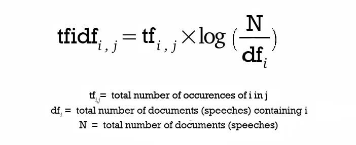
TF-IDF is the value obtained by multiplying the frequency of a given keyword, or Term Frequency, by its Inverse Document Frequency.
Inverse Document Frequency inversely reflects how many documents in the entire collection contain that keyword. Common words receive lower IDF values, while words that appear frequently in a specific document but rarely across the whole corpus receive higher values. The reason for applying a logarithm is to reduce the excessive gap in IDF values as the number of documents grows.
In short, TF represents how often a keyword appears within a document, and IDF represents how rare that keyword is across all documents. A document is represented as a vector composed of TF-IDF values for each word. When a query comes in, we can calculate cosine similarity between the query’s TF-IDF vector and document vectors, then return similar documents.
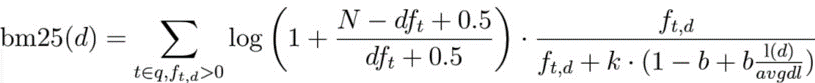
BM25 is a ranking function that improves TF-IDF-based search scores. It improves search result quality by adding document length normalization and smoothing to TF-IDF’s simple frequency-based score.
The left side of the formula is IDF, and the right side is the normalized TF component. f_td is the frequency of term t in document d. The k and b values in the denominator are constant parameters, and the document length l(d) divided by the average document length avgdl is also used for normalization.
In the IDF component, N is the total number of documents, and df_t is the number of documents containing the term. Adding 0.5 avoids cases where the denominator becomes zero. This can be considered a form of smoothing.
From Frequency to Meaning: Dimensionality Reduction Techniques
Linear Discriminant Analysis
One simple dimensionality reduction method used in the 1990s is Linear Discriminant Analysis. This method requires training data with predefined labels for binary classification.
First, it calculates the average position, or centroid, of TF-IDF vectors belonging to one class. It also calculates the average position of TF-IDF vectors in the other class, then draws a line connecting the two centroids. When classifying new data, it takes the dot product between this line vector and the data’s TF-IDF vector to determine which class the data is closer to.
LSA: Latent Semantic Analysis
Latent Semantic Analysis (LSA) is an algorithm that analyzes TF-IDF vectors to extract topics from documents. If Linear Discriminant Analysis is closer to a supervised learning method for binary classification, LSA is an unsupervised learning method that does not require predefined topics.
LSA borrows its idea from PCA (Principal Component Analysis), which is used to reduce the dimensionality of high-dimensional data such as images.
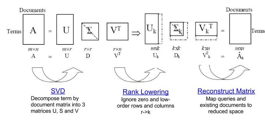
LSA uses Singular Value Decomposition (SVD) to generate a topic-document matrix from a term-document matrix or TF-IDF matrix.
SVD decomposes the original matrix into the product of three matrices. In this decomposition, U and V are orthogonal matrices, while S, or Sigma, is a diagonal matrix. The diagonal elements of S are called singular values. The size of S is connected to the number of topics, and reducing this size results in Truncated SVD.
LDA: Latent Dirichlet Allocation
LDA (Latent Dirichlet Allocation) assumes that a document contains multiple topics in different proportions, and that each word was selected from one of those topics.
For example, suppose we have words like [bicycle, Han River, swimsuit, ocean]. Document 1 could consist of [bicycle, Han River], document 2 of [swimsuit, ocean], and document 3 of [Han River, ocean]. If the topics are [biking, swimming, travel], document 1 could contain multiple topics in proportions such as biking 0.7, swimming 0.1, and travel 0.2.
Conversely, when document 1 contains [bicycle, Han River], we can estimate which topic it is closest to.
First, we set k topics that exist in the document collection. These k topics are assumed to be distributed across documents according to a Dirichlet distribution. Then each word in each document is assigned to one of the k topics. For a word to be classified into the correct topic, we consider both how that word is classified in other documents and how the other words in the same document are classified. Repeating this process across all words in all documents eventually converges to stable values.
Word2Vec
If LSA is closer to understanding the meaning or topic of a document, Word2Vec extracts dense vector representations of individual words. It starts from the assumption that a word’s meaning can be inferred from the words around it.
Word2Vec obtains word vectors using two main methods: Skip-gram and CBOW (Continuous Bag of Words).
For example, suppose we have a sentence like today's lunch is a delicious hamburger. Skip-gram predicts surrounding words such as today's, lunch, and hamburger when delicious is given as input. Conversely, CBOW predicts delicious when today's, lunch, and hamburger are given as input.
What matters when extracting word vectors is not the final output itself, but the hidden layer weights created during training. Since the input is a one-hot vector, the weights affected by that input word can be used as the word vector.
CNN
CNNs (Convolutional Neural Networks), which are mainly used in two-dimensional image domains, can also be applied to text. In text, one-dimensional convolution filters are used to capture local relationships among words.
A convolution filter moves horizontally over a word-vector matrix and performs convolution across the input. This operation multiplies the word embeddings inside the filter by the filter weights, sums the results, and usually applies an activation function such as ReLU. Since each step can be calculated independently, parallel processing is possible.
Each convolution filter produces a different output, and this output is passed as input to the next neural network stage. Dimensionality can then be reduced through pooling, or overfitting can be reduced through dropout. In the final layer, an activation function is applied to represent each data point as a single value. This value is passed to the loss function to calculate error, and the filter weights are updated through backpropagation. Optimizers such as Adam or RMSProp are used to reduce the loss.
RNN and LSTM
CNNs and Word2Vec mostly identify patterns through surrounding words. However, text contains many words that are semantically connected even when they are far apart. To handle this kind of sequential information, RNNs (Recurrent Neural Networks) are used. An RNN passes the output at the current time step t as input to the next time step t+1.
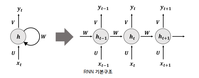
Backpropagation in an RNN is called BPTT (BackPropagation Through Time). It calculates the error between the final output and the target value, then traces backward to determine how much the weights at previous steps contributed. The problem is that as the neural network becomes deeper, vanishing or exploding gradients become more likely.
LSTM (Long Short-Term Memory) is a structure that mitigates these gradient problems while strengthening an RNN’s memory capability. It introduces a state at each step of the neural network, creating a memory that increasingly covers the entire input text as it progresses.
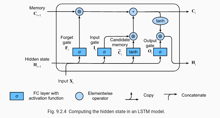
This memory state passes through three gates. The forget gate removes unnecessary memory, and the candidate gate selects components to newly strengthen. Finally, the output gate applies an activation function based on the updated memory vector and input data to produce the output. This output is passed to the next LSTM step.
GRU (Gated Recurrent Unit) is another commonly used structure with a similar purpose.
Seq2Seq and Attention
Seq2Seq refers to an encoder-decoder structure made of LSTMs or GRUs. It feeds input text into the encoder to create a vector, then passes this vector and the expected output values into the decoder to generate results. It is suitable for translation tasks where input and output lengths differ, and because of LSTM characteristics, it can generate variable-length text.
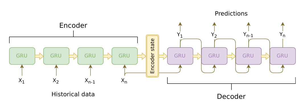
However, Seq2Seq models represent input text as a fixed-size vector. As the text becomes longer, it becomes harder to compress all meaning into a single vector.
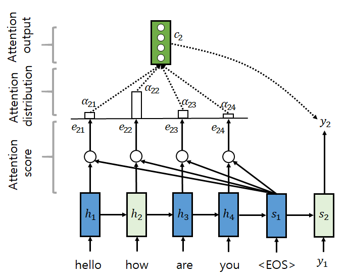
Attention allows the decoder to revisit relevant input words when predicting each output word. In other words, when selecting y_i, it uses the encoder output h_j weighted by the attention weight a_ij. The context vector c_i for y_i can be represented as sum(a_ij * h_j).
Attention scores are calculated using the current decoder output and encoder hidden states, then passed through a softmax function to create a probability vector. This vector and the current decoder output are then used to calculate the next decoder hidden state.
Transformer
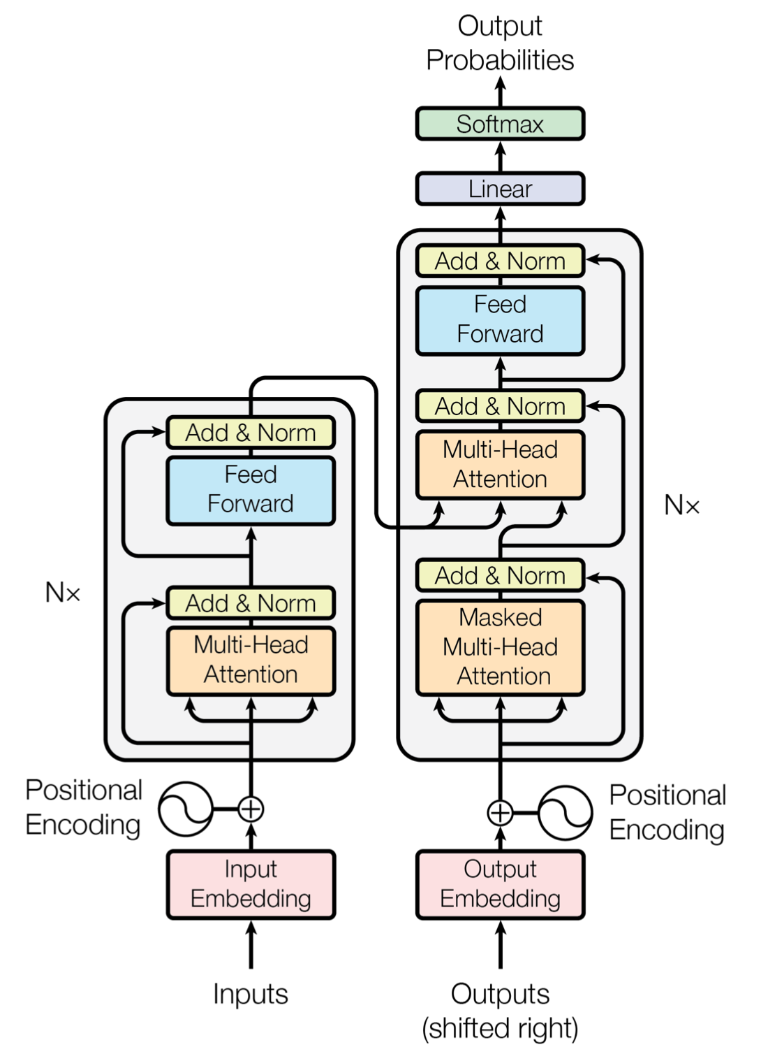
Transformer removes the RNN-based neural networks used in Seq2Seq encoders and decoders, and implements both encoder and decoder using only attention.
However, removing RNNs also removes sequential position information from words. Transformer solves this with Positional Encoding. Positional Encoding adds position information by applying sine functions to even positions of word embedding vectors and cosine functions to odd positions.
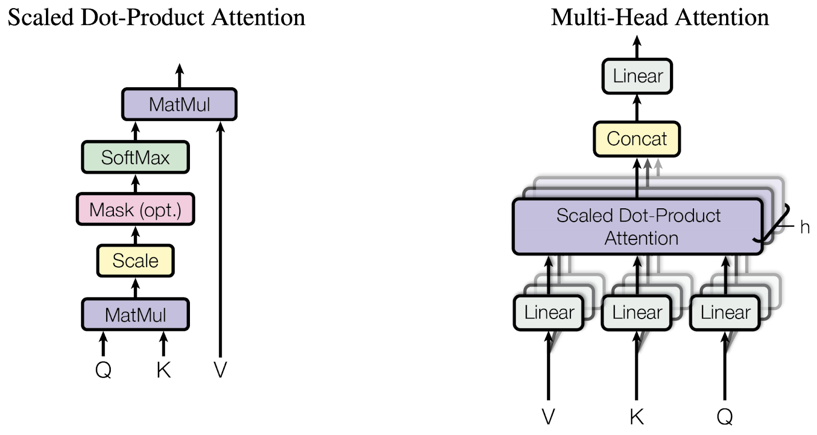
The resulting word embeddings pass through Multi-Head Self-Attention in the encoder. Attention calculates relationships between a specific word’s query and other words’ keys and values. It first takes the dot product between the query and the full key matrix to compute attention scores, then applies softmax to obtain probability values. Multiplying this probability vector by the values produces a value-weighted result representing the relationship between the query and keys.
In the encoder, Q, K, and V are all produced from the same input, so self-attention is performed.
After attention, the data passes through a Feed Forward Network (FFN). The FFN applies ReLU to the first linear layer, then computes the result through a second linear layer. The weights of these linear layers are shared within a single encoder layer, but different layers have different weights.
Add & Norm, located between attention and FFN, refers to residual connection and layer normalization. A residual connection adds the input and output of a function.
The encoder result is then passed to the decoder. The decoder first performs self-attention. Here, the mask prevents the model from referring to target words after the current time step by assigning very small values to future positions.
The decoder’s second attention uses the encoder outputs as key and value, and the decoder values as query, allowing it to refer to encoder information. The same process is then repeated to produce the final output.
Summary
TF-IDF and BM25 compare text based on word frequency and importance within documents. LSA and LDA attempt to discover hidden topics in documents, and Word2Vec represents words themselves as meaningful vectors. CNNs, RNNs, and LSTMs are neural network-based approaches for learning patterns and sequence in text.
Finally, Attention and Transformer learn which words to treat as more important in long contexts, and evolved in a direction that reduces the burden of sequential computation. The flow of NLP ultimately leads to the question: “How do we turn text into numbers, and how do we learn meaningful relationships among those numbers?”
References
- Natural Language Processing in Action with Python, 2020
- https://wikidocs.net/book/2155
- https://m.blog.naver.com/ckdgus1433/221608376139
- https://d2l.ai/chapter_recurrent-modern/lstm.html
- http://incredible.ai/nlp/2020/02/20/Sequence-To-Sequence-with-Attention/